≡ Menu

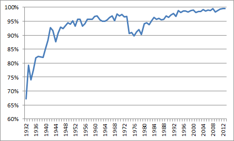
In terms of NFL averages, completion percentage is way up, interception rate is way down, pass attempts are way up, and the passing game has never been more valuable. We all know that. But sometimes, when everyone is zigging, a lone team might be better off zagging.

The question here is does that theory apply to trying to build an offense that revolves around a power running game? Defenses are looking for lighter and faster defensive ends and linebackers who can excel in pass coverage; just about every defense is taking linebackers off the field for defensive backs more than they did a decade ago. And defenses spend the majority of their practice reps focusing on stopping the pass, too. As defenses try to become faster, quicker, and lighter — and better against the pass — should a team try to respond by developing a power running game?

On one hand, it’s tempting to say of course that model could work: just look at the Seahawks and Cowboys. Seattle does have a dominant running game, of course; what the Seahawks did to the Giants last year is not safe for work. But Seattle also has Russell Wilson, perhaps the most valuable player in the league when you combine production, position, and salary. And the best defense in the NFL. So yes, the Seahawks are successful with a power running game, but that’s not really a model other teams can follow. And for all the team’s success, Seattle doesn’t even have a very good offensive line, which would seem to be the number one focus for a team that is trying to build a power running attack.

The team with the best offensive line in the NFL is probably in Dallas. But the Cowboys also have Tony Romo and Dez Bryant, so again, that’s not really a model capable of imitation.

I’m thinking about some of the teams in the middle class of the AFC — the Bills, the Jets, the Browns, the Texans — teams that are currently trying the all defense, no quarterback approach. Finding a quarterback is the most difficult thing there is to do in the NFL, and these four teams can attest to that. By trading for LeSean McCoy, it appears as though Buffalo is trying to do what this article implies, but there are two problems with that plan. One, the Bills have one of the worst offensive lines in the NFL, and two, McCoy is not necessarily the right guy to build a move-the-chains style of offense.

The Jets have invested a ton of money in their offensive line, courtesy of hitting on first round draft picks in 2006 with Nick Mangold and D’Brickashaw Ferguson, and spending to acquire mid-level free agents from Seattle (James Carpenter this year after Breno Giacomini last offseason). But the Jets offensive line is far from dominant, and the team isn’t really building around a power running game (the team’s top two tight ends are below-average blockers, and the Jets are investing more in wide receivers than running backs).

Houston is an interesting case, because the Texans led the NFL in rushing attempts last year. The Texans do have a very good run-blocking offensive line and Arian Foster, but it still feels like that’s just not enough. Houston’s efficiency numbers were harmed by giving carries to Alfred Blue — the Texans were 8-5 when Foster was active — but the team also doesn’t have much in the way of run blockers at tight end or fullback. [continue reading…]

{ 22 comments }

Re-Post: Data Snooping

In lieu of weekend trivia, I am going to begin reposting old articles that I think people would still find relevant. If you’re a new reader, I hope you enjoy; if you’re an old-timer, my hunch is you still will get something new out of reading these again, just like I did. Today’s post is on Data Snooping, originally posted by me in June 2013.


Reggie Wayne dominates when seeing blue

Reggie Wayne dominates when seeing blue.

Over the last few years, the football analytics movement has made tremendous progress. There are many really smart people with access to a large amount of useful information who have helped pioneer the use of statistics and analytics in football. Major news organizations and NFL teams seem to be embracing this movement, too. Unfortunately, there are some less-than-desirable side effects as the reward for presenting “statistical information” seems larger than ever.

Data snooping is the catch-all term used to describe a misuse of data mining techniques. There are perfectly legitimate uses to data-mining, but data snooping is a big ‘no-no’ for the legitimate statistician. If the researcher does not formulate a hypothesis before looking at the data, but instead uses the data to suggest what the hypothesis should be, then he or she is data snooping. [continue reading…]

{ 0 comments }

In 2013, eight teams hired new head coaches.  Three teams tapped rising offensive coordinators – Mike McCoy, Bruce Arians, [1]Who, of course, was also coming off an award-winning season as interim head coach of the Colts. Rob Chudzinski – while four other hires were head coaches with offensive backgrounds (Andy Reid, Doug Marrone, Chip Kelly, and Marc Trestman).  That means just one head coaching hire came from a defensive background: Gus Bradley in Jacksonville.

Given the current era where the rules are slanted towards the offense, one can understand how teams might be inclined to look towards offensive coaches when selecting a head coach. Consider that scoring is about 60% of the game, which could make owners and general managers break ties in favor of offensive candidates. Then, remember that the pool of teams looking for a new head coach: teams that struggled the prior year. And since offense is so important, that usually means a team that had a bad offense. It’s a bit of an oversimplification, but it’s easy to imagine the average team looking for a head coach as one that just went 5-11 with a bad offense and is looking to turn things around with a new, sexy offensive hire.

There was something else you may recall from 2013: the lack of minority hires. At the end of the 2012 season, there were 15 job openings for general managers and head coaches; none went to a minority candidate. The hiring process for GMs is much more opaque than it is for head coaches, but there was one main explanation given for the fact that all 8 head coaching hires were white: black coaches are disproportionately defensive coaches, and the league was shifting towards offense when it came to coaching hires because of the reasons stated above. [continue reading…]

References

References
1 Who, of course, was also coming off an award-winning season as interim head coach of the Colts.
{ 4 comments }

Are NFL Playoff Outcomes Getting Less Random?

In September 2012, Neil Paine wrote a great article at this website titled: Are NFL Playoff Outcomes Getting More Random? In it, Neil found that randomness had increased significantly in the NFL playoffs, with “recently” defined as the period from 2005 to 2011.

In fact, while 2005 was a pretty random postseason, 2006 was one of the more predictable playoff years.  But the five-year period from 2007 to 2011 was a really random set of years. Consider that:

  • In 2007, the Giants won three games as touchdown underdogs, including the Super Bowl as a 12.5-point underdog.  The Chargers also won a playoff game against the Colts as an 11-point dog.
  • In 2008, five of the eleven playoff games were won by underdogs! That list was highlighted by the Cardinals winning in Carolina as a 10-point underdog in the divisional round.
  • The following year, five of the eleven playoff games were upsets, including the Jets winning as 9-point underdogs in San Diego.
  • In 2010, for the third straight year, there were five playoff upsets, including two huge ones: the Jets as 9.5 point dogs in Foxboro, and the Seahawks as 10-point home dogs against the Saints.
  • Noticing a trend? Well, in 2011, five of the playoff games were again won by the underdog. The two big upsets here were the Tim Tebow-led Broncos against the Steelers, and the Giants winning in Lambeau Field against the 15-1 Packers.

[continue reading…]

{ 10 comments }

Guest Post: Are Interceptions Overrated?

Guest contributor Adam Steele is back again. You can read all of Adam’s articles here.


Are Interceptions Overrated?

There’s nothing worse than throwing an interception. Everyone seems to agree on this, from fans to media to advanced stats guys. But is it really true? In this quick study, I looked at the tradeoff between interception avoidance and aggressive downfield passing to see which strategy has a larger impact on winning. To measure this, I created two categories of quarterbacks: Game Managers and Gunslingers.

First, the Game Managers, which includes all post-merger quarterback seasons with an INT%+ of at least 110 [1]Which means the player was at least 0.67 standard deviations better than league average at avoiding interceptions. and a NY/A+ of 90 or below (min 224 attempts). [2]Which means the player was at least 0.67 standard deviations worse than league average in net yards per attempt. These guys avoided picks but failed to move the ball efficiently, the hallmark of a conservative playing style.

[continue reading…]

References

References
1 Which means the player was at least 0.67 standard deviations better than league average at avoiding interceptions.
2 Which means the player was at least 0.67 standard deviations worse than league average in net yards per attempt.
{ 27 comments }

Betting Bad: Thinking About Uncertainty in Prediction

Barack Obama was not the only winner in the 2012 presidential election. Nate Silver, now founder and editor in chief of Five Thirty Eight, and other stats-y election forecasters basked in the praise that came when the returns matched their predictions.

But part of the praise was overstated. At the very end, Silver’s models essentially called Florida a toss-up, with the probability of an Obama win going just a few tenths of a percentage point above 50%. But because his model gave Obama the slightest of edges in Florida, his forecast in most of the media essentially became a predicted Obama win there. In addition to accurately forecasting the national popular vote, Silver then received credit for predicting all fifty states correctly.

I am all in favor of stats winning, but the flip side of this is the problem. If Obama had not won Florida, Silver’s prediction―which, like that of other forecasters such as Sam Wang of the Princeton Election Consortium, was excellent―would have been no less good. [1]This is a column about football, but you might want to check out some of the stuff through that link on the differences between Silver and Wang on the upcoming midterm elections. They both know way … Continue reading And if stats folks bask too much in the glow when everything comes up on the side where the probabilities leaned, what happens the next time when people see a 25% event happening and say that it invalidates the model? [2]Of course, maybe Football Outsiders has already run into that with the 2007 Super Bowl prediction. Perhaps sports people are ahead of politics on this stuff.

Lots of people have made this point before — heck, Silver wrote about this in his launch post at the new 538 — but it is really useful to think carefully about the uncertainty in our predictions. Neil has done that with his graphs depicting the distribution of team win totals at 538, and Chase did so in this post last Saturday. Football Outsiders does this in its Almanac every year, with probabilities on different ranges of win totals. [continue reading…]

References

References
1 This is a column about football, but you might want to check out some of the stuff through that link on the differences between Silver and Wang on the upcoming midterm elections. They both know way more than I do, but for the small amount that it is worth, I lean more towards Wang on this one.
2 Of course, maybe Football Outsiders has already run into that with the 2007 Super Bowl prediction. Perhaps sports people are ahead of politics on this stuff.
{ 12 comments }

Super Bowl Champions and Top-Heavy Divisions

The NFL realigned its divisions in 2002, placing four divisions of four teams each in each conference. Some divisions have been top-heavy, with the most obvious example being the 2007 AFC East. The Patriots won 16 games, while the Jets, Dolphins, and Bills combined to win just twelve games (with six of those twelve wins by the Bills or Jets against the Dolphins or Jets). That means New England was responsible for 57% of all wins by AFC East teams in 2007, easily the highest percentage of any team in a division since realignment.

Having an easy division brings some advantages: being the best team in a bad division makes it easier to get the best record in the conference, which leads to a bye week and home field advantage.  It also could allow a team to rest its starters at the end of the year.  Conversely, there’s the notion that teams in tough divisions “beat up on each other,” so presumably that’s another benefit to being the best team in a bad division.

But New England, of course, didn’t win the Super Bowl in ’07.  That year, the title went to the NFC East, which was not a top-heavy division; the Cowboys had just 33% of NFC East wins that year, placing it as the 3rd least top-heavy division in the NFL.  The last three years, things have been even more stark:

  • The NFC West was one of the strongest divisions in NFL history last year; but while the Seahawks may have been beaten up by the 49ers, Cardinals, and Rams, that didn’t stop Seattle from winning the Super Bowl.  Seattle won “just” 31% of the games won by the NFC West last year — only the NFC North (Green Bay, 29%) was less top-heavy.
  • The least top-heavy division in football in 2012 was the AFC North. Baltimore won 10 games, but so did Cincinnati, and the Steelers (8) and Browns (5) were not pushovers, either. The Ravens won just 30% of all games won by AFC North teams in 2012, but finished the year by hoisting the Lombardi Trophy.
  • In 2011, the Giants won a competitive NFC East with a 9-7 record; Philadelphia and Dallas were just one game behind, and New York won only 30% of all games won by NFC East teams that year. Only the Tim Tebow-infected AFC West was less top-heavy (Denver won 26% of all AFC West games, just barely above the minimum threshold for a division champ) that year.

The graph below displays all eight divisions for each year since 2002.  The Y-axis shows the percentage of games won by the top team in the division as a percentage of the total wins by that division.  The X-axis represents the year; the red dot represents the division with the eventual Super Bowl champ, with the blue dot for all other divisions. [continue reading…]

{ 8 comments }

Let’s get the disclaimer out of the way: the traditional draft value chart is outdated, and it never made much sense in the first place. Trying to use logic to explain why teams operate in an illogical manner is a tall task, and probably a waste of time. So, let’s try anyway.

First, I recreated my draft value chart. To do that, I looked at the first 224 players selected in each draft from 1970 to 2009. PFR assigns Approximate Value grades to each player in each season, but since AV grades are gross units, we need to tweak those numbers to measure marginal value. As a result, I only gave players credit for their AV above two points in each season; that difference is a metric I’m defining as a player’s Marginal AV. For example, if a player has AV scores of 8, 1, and 3 in three straight years, those scores are translated into Marginal AV scores of 6, 0 and 1.

The graph below shows the average Marginal AV produced by each draft pick in each season from ’70 to ’09. The blue line shows the average Marginal AV produced by draft picks as rookies, the red line represents second-year players, green is for year three, purple for the fourth season, and orange for average Marginal AV in year five. [continue reading…]

{ 8 comments }

xp avgThe NFL’s Competition Committee is currently considering rules changes to eliminate the boredom associated with the extra point. As you can see from the graph above, extra points are practically automatic now, to the tune of a 99.6% conversion rate in 2013. In fact, extra points have been close to automatic for awhile; the success rate was even as high as 96.8% in 1973, the last year the goal posts were still right on the goal line. The conversion rate was depressed for about 15 years before bouncing back to 97% in 1989, and there have been just 18 missed extra points total in the last three years. I don’t disagree that something could be done to improve the quality of the game.

The simplest alternative is to make touchdowns worth seven points instead of six, and to allow a team to gamble one of those points in the hopes of getting two points by “going for two.” In other words, we would have the system we have now, except that the song and dance of actually kicking the extra point is replaced with an automatic point.

Another solution is to eliminate the extra point entirely, requiring that teams go for two after every touchdown. I won’t try to answer the subjective question of whether or not this would make for a more enjoyable fan experience; the more interesting question to me is whether or not this would lead to more upsets. In other words, if teams had to go for two after every touchdown, would this lead to the better team winning more or less often? I posed this question on the Footballguys.com message boards and got into a good discussion there, much of which I’ll summarize here.

Before analyzing, we must recognize that the two-point play is not like a typical NFL play. A team that’s great in short yardage (say, Carolina) would probably be better off than most teams at converting on these attempts. Likewise, teams that excel in goal-line defense but maybe don’t have great corners (like say, Carolina) would probably be better off, too. But I think, on average, good teams are better at converting two point plays than bad teams, and, on average, good teams are better at preventing two point conversions than bad teams.

So how would such a rule change impact NFL games? One argument that this rule change would make the better team more likely to win is that this would present an additional hurdle for the weaker team. By replacing a play where everyone is successful with a competitive play, this increases the sample size, generally a bad thing for underdogs. Right now, a weaker team only needs to match the stronger team touchdown for touchdown (and field goal for field goal and safety for safety). But if the weaker team matches the better team under this new regime, the weaker team, on average, will still be trailing. By increasing the sample size of relevant plays, the weaker team needs to outplay the better team for longer, making it harder to pull the upset.

On the other hand, the argument is probably more convincing the other way that a mandatory “go for two” rule would lead to more upsets. That’s because the 2-point conversion play is a high-leverage play, and the inclusion of more high-leverage plays is generally a positive circumstance for the underdog. Imagine a rule change where the NFL made going for 2 mandatory, but made the successful outcome worth 20 points. That environment would almost certainly make things better for weaker teams: instead of having to outplay the better team for 60 minutes, the weaker team could be outplayed and win as long as they won on two or three key plays. That’s taking the example to its extreme, but one could argue that the same idea holds with the conversion worth two points, even if the effect would obviously be muted.

Here’s another way to think about it.  Let’s ignore games that aren’t very competitive, because the outcomes of those games won’t change under the current format or the “mandatory go for two” environment.  But there are three other types of games: [continue reading…]

{ 10 comments }

When will a team go an entire game without running?

Belichick checks to see if anyone has gone a whole game without calling a run yet

Belichick checks to see if anyone has gone a whole game without calling a run yet.

The record for fewest rush attempts in a game is 6, set by the 2004 Patriots and tied by the ’06 Cardinals. The circumstances there are as you would expect. The Patriots fell behind 21-3 in the first quarter to the Steelers in 2004, and Pittsburgh owned the league’s top rush defense. In 2006, the Cardinals faced the Minnesota Vikings, owners of one of the greatest rush defenses in history. Minnesota allowed just 985 yards (the second lowest in modern history) on 2.8 yards per carry (the third lowest mark of the modern era) in 2006. That day, the Cardinals didn’t fall behind early, but called on Matt Leinart to throw 51 passes compared to just four Edgerrin James runs. It was not a winning formula, but I’m not sure Denny Green had the wrong strategy.

But will a team ever go a full game without attempting a run? In college, the floor has also been six runs, at least in recent memory. Baylor — with coach Guy Morris, who coached under Hal Mumme and next to Mike Leach at both Valdosta State and Kentucky — was the first, calling just six runs on the road against the 2006 Texas Longhorns. A year later in Austin, it was Leach who orchestrated the only other six-carry game since 2005. That day, he put the game in the hands of Graham Harrell (36/48, 466 yards, 5 TDs, 1 INT), Michael Crabtree (9/195/2), Danny Amendola (8/82) and Edward Britton (8/125/1), but alas, the Red Raiders defense couldn’t stop Jamaal Charles.

I suppose we should wonder when the first 5-carry game will occur before asking about the first 0-carry game. But it’s a Sunday in the offseason, so I’ll throw this one out to the crowd. Will we ever see a 0-carry game? If so, how many years from now until it occurs? Against the Bills this year, the Ravens called 31 straight passing plays but still passed on “only” 86% of all plays from scrimmage. What will it take to get that percentage to 100?

{ 15 comments }

Insane Ideas: Rules Changes

Should the depth of the NFL end zone be extended from 10 to 20 yards? Practically, this is probably impossible, as adding 20 yards to certain fields would be an issue in many NFL stadiums. But let’s ignore that issue for today. I recently had lunch with a baseball friend of mine who suggested this change. My initial reaction was that this would be a bit odd, but there are several reasons to like his idea:

1) My baseball friend — let’s just call him Sean — doesn’t like how compressed things are at the goal line. Why are teams in effect penalized for getting down to the 1 yard line? Why make things easier on the defense?

If you think about it, there’s no reason for the end zone to be ten yards deep. If you are someone who believes we need more rules to promote defense, would you be in favor of making the end zone five yards deep? If not, why not? What makes ten the right number?

We have been conditioned by announcers to believe that life is tougher near the goal line for NFL offenses, and that this is a good thing. Does that make sense?

2) The goal posts would remain at the back of the end zone, which has three benefits. One, the extra point would now be slightly more difficult, which would quiet that controversy. Two, teams might be a little more likely to go for it on 4th and goal, as a 30-yard field goal isn’t as much of a gimme as a 20-yarder. But most importantly, when it’s fourth-and-three from the 30 yard line, teams would now go for it. Perhaps idiot-proofing coaching isn’t a desirable reason for change, but I am in favor of most rules that result in less kicking.

3) This would allow for 119-yard returns, a trade-off that I’m willing to make even if it lowers the possibility of an Orlovsky happening.

So what do you guys think? Feel free to leave your thoughts in the comments, or go in a different direction and post your own insane idea rules change. Here’s one of mine: in the final two minutes of the fourth quarter, the clock stops on a play that does not gain yards.

The purpose of this hypothetical rule change would be to stop teams from taking a knee to end the game. I don’t expect this to be a very popular idea, although the Pro Bowl actually implemented this rule this year. But watching teams battle for 58 minutes and then have the game essentially end with 2 minutes left always rubbed me the wrong way. I know, I know, the winning team earned the right to do it. That doesn’t mean I have to like it. I’d rather see a team have to at least gain a yard to end the game. I’m pretty sure all 32 coaches would hate this rule, but it would certainly make the end of certain games more exciting. That’s a pretty risky statement, I know, because it’s hard to top the victory formation for excitement.

{ 44 comments }

One of my favorite sabermetric baseball articles of all time was written by Sky Andrecheck in 2010 — part as a meditation on the purpose/meaning of playoffs, and part as a solution for some of the thorny logical concerns that arise from said mediation.

The basic conundrum for Andrecheck revolved around the very existence of a postseason tournament, since — logically speaking — such a thing should really only be invoked to resolve confusion over who the best team was during the regular season. To use a baseball example, if the Yankees win 114 games and no other AL team wins more than 92, we can say with near 100% certainty that the Yankees were the AL’s best team. There were 162 games’ worth of evidence; why make them then play the Rangers and Indians on top of that in order to confirm them as the AL’s representative in the World Series?

Andrecheck’s solution to this issue was to set each team’s pre-series odds equal to the difference in implied true talent between the teams from their regular-season records. If the Yankees have, say, a 98.6% probability of being better than the Indians from their respective regular-season records, then the ALCS should be structured such that New York has a 98.6% probability of winning the series — or at least close to it (spot the Yankees a 3-0 series lead and every home game from that point onward, and they have a 98.2% probability of winning, which is close enough). [continue reading…]

{ 8 comments }

Is that Bayes?

Is that Bayes?

Peyton Manning is not a 51 touchdown per-season quarterback, but that doesn’t mean he won’t average the necessary 2.9 touchdowns per game over his final ten games this season to break Tom Brady’s touchdown record. Before the season, Footballguys.com projected Manning as a 2.38 passing touchdown per game player.  And while he has looked unstoppable thus far, with 22 touchdown throws in six games, Manning has been known to have great spurts before, too.  All quarterbacks have hot and cold streaks, Manning included.  From 2003 to 2012, after removing games where he sat late in the season, Manning averaged 2.17 passing touchdowns per game with a standard deviation of 1.31 touchdowns. [1]That was after removing week 17 of the ’04, ’05, ’07, ’08, and ’09 seasons, and week 16 of the ’05 and ’09 seasons, when Manning left early. Why did I pick the last ten years? I don’t … Continue reading  In the ’04 season, Manning threw at least 20 touchdowns in each of his trailing six game stretches from week 7 all the way through week 15, with a peak of 27 touchdowns in his prior six games in weeks 11 and 12.  Manning also threw 19 touchdowns in his last two full regular season games of 2010 and his first four games of 2011.  White-hot streaks happen, even to the best players, so we shouldn’t just assume that he’s now a 3.67 touchdown per game player.

On the other hand, it would be naive to assume that we should ignore the first six weeks of the season and continue to project Manning as a 2.38 touchdown per game player for the rest of the year.  The question becomes, how much do we base projection over the final 10 games on his preseason projection and how much do we base it on his 2013 results? In Part I, after four games, a regression model produced a projection of 2.56 touchdowns per game the rest of the year. But the problem with a regression analysis is that Manning is an extreme outlier among NFL quarterbacks; to project Manning, it would be best if we could limit ourselves to just quarterbacks named Manning Peyton Manning.

Before continuing, I want to give a special thanks to Danny Tuccitto, without whom this article wouldn’t be possible. Danny provided this great link and also spent a lot of time walking me through the process. To the extent I’ve mucked it up here, you should blame the student, not the teacher. But after walking through some models online, I realized that the best explanation about how to use Bayes Theorem for these purposes was on a sweet site called FootballPerspective.com. And the smartest person on that website had already laid out the blueprint.

In the comments to one of his great posts, Neil explained that we can calculate Manning’s odds using Bayes Theorem if we know four things:

His Bayesian prior mean (i.e., his historical average):

His Bayesian prior variance (the variance surrounding his historical average):

His observed mean:

His observed variance:

Let’s go through each of these:

1) Manning’s Bayesian prior mean: this is simply what we expected out of Manning before the season. I will use 2.38, since Footballguys is the gold standard of football projections in my admittedly biased opinion. But you can use any number you like, as I’ll provide the full formula at the end.
[continue reading…]

References

References
1 That was after removing week 17 of the ’04, ’05, ’07, ’08, and ’09 seasons, and week 16 of the ’05 and ’09 seasons, when Manning left early. Why did I pick the last ten years? I don’t know, but he won his first MVP in ’03, so that seemed like a useful starting point.
{ 9 comments }

“Worldly wisdom teaches that it is better for the reputation to fail conventionally than to succeed unconventionally.” – John M. Keynes.

Photo via phillymag.com.

Last Thursday night, Chip Kelly was widely criticized for an unconventional decision that turned out to be unsuccessful. Trailing 10-0 in the first quarter against the Chiefs, Michael Vick threw a 22-yard touchdown pass to Jason Avant. The photo above shows how the Eagles lined up for the point after. Philadelphia’s two-point conversion attempt — a play known as the the Swinging Gate — was stopped, and it was stopped in particularly ugly fashion. That made it easy to point a finger and laugh at the college coach doing something silly.

But without the benefit of hindsight, there was nothing silly or even suboptimal about the decision. Putting aside the specifics of the play — we’ll get to that at the end — the main criticism seems to be that it was “too early” to go for two, or that the Eagles were “chasing points”, or that it was simply “unnecessary.” All of those are buzz words for saying that the Eagles should have behaved conventionally.

At a baseline level, let’s recognize that a team has a roughly 50/50 chance of converting on a two-point conversion. For a good offense with a mobile quarterback, that number may be even higher, but let’s just use the 50/50 number now. If that’s the case, then teams early in the game should be indifferent between kicking the extra point and going for two. Consider this hypothetical example: if a team had the option of kicking the extra point or flipping a coin — and heads gave them two points, tail giving them zero — would choosing to flip the coin be a poor decision?

Late in games, perhaps. But early in the game? I don’t see any reason to think that the difference between having six versus seven points on the board in the first quarter is more significant than the difference between having seven or eight points. Suppose you were told that your favorite team would score first quarter touchdowns in back-to-back games. Option 1 provides that your team would the extra point both times, while Option 2 is that your team would make the two point conversion once and fail on the attempt once. So you get eight points in one game and six points in the other.

Which would you prefer, Option 1 or Option 2? And why? And, if you prefer Option 1 to Option 2, how much more preferable is it? What would you be willing to trade to land in Option 1 — how many yards on the ensuring kickoff?

I would be indifferent between Options 1 and 2, but even if you preferred one, I don’t see how anyone could strongly prefer Option 1 to Option 2. The value to having 8 points is real, which is why it is never “too early” or “unnecessary” to go for two in a world where teams convert on two-point attempts half the time. Those are red herrings, because going for two is only a high-variance strategy; is it not a high-variance, lower-expected value option. Once you understand that, then nearly all the criticism about Kelly’s decision disappears.

As for the actual play call? I think it was a good one. Keep in mind that the Eagles did not pigeon hole themselves into going for two — based on how the Chiefs reacted to that formation prior to the snap, Philadelphia could have switched back to a normal extra point formation or simply taken a delay of game penalty with minimal harm. But Kansas City did not react well to the play pre-snap: The Eagles split two players out wide to the right, and Kansas City countered with two defenders to that side. But in the middle of the field, Philadelphia had the snapper, holder, and kicker, while the Chiefs kept four players in the middle of the field. I’m quite certain the special teams coach was not pleased with how the Chiefs responded to the situation, because that left K.C. with only five defenders to the defense’s right, while the Eagles were able to match up five blockers to that side and Zach Ertz, the eventual ballcarrier.

That’s a matchup Philadelphia should win more often than fifty percent of the time, and perhaps significantly more often than that. As it turns out, Lane Johnson blew the block, Tamba Hali made a nice play, and Kelly and the Eagles had egg on their face. Failing unconventionally has its drawbacks.

{ 4 comments }
Spoiler: the quarterback plays a big role in passing yards.

Spoiler: the quarterback plays a big role in passing yards.

In May, I wrote that the scoring team is responsible for roughly 60% of the points it scores, while the opponent is responsible for 40% of those points. In other words, offense and defense both matter, but offense tends to matter more.

I was wondering the same thing about passing yards. When Team A plays Team B, how many passing yards should we expect? As we all know, Team A can look very different when it has Dan Orlovsky instead of Peyton Manning, so I instead chose to look at Quarterback A against Team B. Here’s the fine print:

1) I limited my study to all quarterbacks since 1978 who started at least 14 games for one team. Then, I looked at the number of passing yards averaged by each quarterback during that season, excluding the final game of every year. I also calculated, for his opponent, that team’s average passing yards allowed per game in their first 15 games of the season.

2) I then calculated the number of passing yards averaged by each quarterback in his games that season excluding the game in question. This number, which is different for each quarterback in each game, is the “Expected Passing Yards” for each quarterback in each game. I also calculated the “Expected Passing Yards Allowed” by his opponent in each game, based upon the opponent’s average yards allowed total in their other 14 games.

3) I then subtracted the league average from the Expected Passing Yards and Expected Passing Yards Allowed, to come up with era-adjusted numbers.

4) I performed a regression analysis using Era-Adjusted Expected Passing Yards and Era-Adjusted Expected Passing Yards Allowed as my inputs. My output was the actual number of passing yards produced in that game.
[continue reading…]

{ 10 comments }

Fast and Faster

Fast and Faster.

The number one storyline in the NFL in week one isn’t the health of Robert Griffin III, but the presence of two other men occupying FedEx Field that night. The football world is anxiously awaiting to see how Chip Kelly’s offense, piloted by Michael Vick, will work in the NFL. We don’t know much, but we do know that the coach plans to incorporate the fast-paced, up-tempo style that his teams used at Oregon to obliterate opponents.

In May, I took a stab at discussing tempo in the NFL, and I presented a couple of lists that measured the number of plays run per second of possession in the NFL. Today, I want to revisit the questions of tempo and pace using more precise measurements.  Let’s start with some league-wide data. The table below shows the average number of seconds between snaps for NFL teams last season. I’ve excluded a number of plays from this sample, including all plays at the start of a quarter, all overtime plays, plays after a changes of possession, and plays in the final three minutes of the first half or five minutes of the second half (where teams are less likely to operate at their normal pace).

secs btw plays
[continue reading…]

{ 8 comments }

Last night, David Wilson ran 84 yards for a touchdown on the Giants first play from scrimmage. Without being touched. How does that happen? Let’s start with a look from the end zone right at the snap:

Giants Jets Wilson Snap

The Jets are lined up with four down linemen: from left to right, you can see DE Muhammad Wilkerson, first-round tackle Sheldon Richardson, backup NT Damon Harrison, and outside linebacker/edge rusher Garrett McIntyre. At linebacker, we see Calvin Pace, David Harris, and Demario Davis — the new starter whom Rex Ryan has compared to Ray Lewis — tight inside the tackles. Left cornerback Kyle Wilson is off screen, covering Rueben Randle on the Giants right, while the Jets show a single-high safety look: Dawan Landry, the free agent addition from Jacksonville, is 13 yards off the line of scrimmage, while safety Antonio Allen (the Jets 7th round pick a year ago and expected starter in 2013) has creeped towards the line. What’s not shown: a few seconds earlier, the Giants motioned TE Brandon Myers to the offense’s left before the snap, causing Antonio Cromartie to line up right in the face of Hakeem Nicks and Allen (39) to drop down closer to the line of scrimmage (he was ten yards off the line before Myers moved).

The Giants know what is coming: a handoff to David Wilson, who will read the Jets defense to determine whether he bursts up the gut or bounces outside. From a numbers game, the Giants like what they see: even after Allen comes down, the math looks even. Assuming Nicks can handle Cromartie (he will), the Giants have the center, left guard, left tackle, Myers (a yard off the line) and TE Bear Pascoe (playing the traditional fullback slot) to block five Jets – Harrison and McIntyre on the line, Harris and Davis in the second level, and Allen.

In theory, you would think the Giants would have the C block the NT, the uncovered LG would make a beeline towards Harris (52), the LT would take care of McIntyre, and Pascoe and Myers would be assigned to Davis (56) and Allen (39). Some of that happens — the center (backup Jim Cordle) handles the nose; he also gets an assist from LG Kevin Boothe, who nudges Harrison away from the play a second before he manhandles Harris (a mismatch for most linebackers, so we can’t be too harsh on Harris). LT Will Beatty also overpowers the RDE, McIntyre, unsurprising considering (1) Beatty is a pretty good player and McIntyre is a backup 3-4 OLB, and (2) Beatty outweighs him by 64 pounds. Credit the Giants for good blocking, but blocking your assigned man doesn’t turn into 84-yard runs very often. The real cuprit on the play is Allen, but he was only the last domino to fall.
[continue reading…]

{ 5 comments }

Last week, I wrote about why I was not concerned with Trent Richardson’s yards per carry average last season. I like using rushing yards because rush attempts themselves are indicators of quality, although it’s not like I think yards per carry is useless — just overrated. One problem with YPC is that it’s not very stable from year to year. In an article on regression to the mean, I highlighted how yards per carry was particularly vulnerable to this concept. Here’s that chart again — the blue line represents yards per carry in Year N, and the red line shows YPC in Year N+1. As you can see, there’s a significant pull towards the mean for all YPC averages.

regression ypc

I decided to take another stab at examining YPC averages today.  I looked at all running backs since 1970 who recorded at least 50 carries for the same team in consecutive years. Using yards per carry in Year N as my input, I ran a regression to determine the best-fit estimate of yards per carry in Year N+1. The R^2 was just 0.11, and the best fit equation was:

2.61 + 0.34 * Year_N_YPC

So a player who averages 4.00 yards per carry in Year N should be expected to average 3.96 YPC in Year N+1, while a 5.00 YPC runner is only projected at 4.30 the following year.

What if we increase the minimums to 100 carries in both years? Nothing really changes: the R^2 remains at 0.11, and the best-fit formula becomes:

2.63 + 0.34 * Year_N_YPC

150 carries? The R^2 is 0.13, and the best-fit formula becomes:

2.54 + 0.37 * Year_N_YPC

200 carries? The R^2 stays at 0.13, and the best-fit formula becomes:

2.61 + 0.36 * Year_N_YPC

Even at a minimum of 250 carries in both years, little changes. The R^2 is still stuck on 0.13, and the best-fit formula is:

2.68 + 0.37 * Year_N_YPC

O.J. Simpson typifies some of the issues. It’s easy to think of him as a great running back, but starting in 1972, his YPC went from 4.3 to 6.0 to 4.2 to 5.5 to 5.2 to 4.4. Barry Sanders had a similar stretch from ’93 to ’98, bouncing around from 4.6 to 5.7 to 4.8 to 5.1 to 6.1 and then finally 4.3. Kevan Barlow averaged 5.1 YPC in 2003 and then 3.4 YPC in 2004, while Christian Okoye jumped from 3.3 to 4.6 from 1990 to 1991.

This guy knows about leading the league

This guy knows about leading the league.

Those are isolated examples, but that’s the point of running the regression. In general, yards per carry is not a very sticky metric. At least, it’s not nearly as sticky as you might think.

That was going to be the full post, but then I wondered how sticky other metrics are.  What about our favorite basic measure of passing efficiency, Net Yards per Attempt? For purposes of this post, an Attempt is defined as either a pass attempt or a sack.

I looked at all quarterbacks since 1970 who recorded at least 100 Attempts for the same team in consecutive years. Using NY/A in Year N as my input, I ran a regression to determine the best-fit estimate of NY/A in Year N+1. The R^2 was 0.24, and the best fit equation was:

3.03 + 0.49 * Year_N_NY/A

This means that a quarterback who averages 6.00 Net Yards per Attempt in Year N should be expected to average 5.97 YPC in Year N+1, while a 7.00 NY/A QB is projected at 6.45 in Year N+1.

What if we increase the minimums to 200 attempts in both years? It has a minor effect, bringing the R^2 up to 0.27, and producing the following equation:

2.94 + 0.51 * Year_N_NY/A

300 Attempts? The R^2 becomes 0.28, and the best-fit formula is now:

2.94 + 0.53 * Year_N_NY/A

400 Attempts? An R^2 of 0.26 and a best-fit formula of:

3.18 + 0.50 * Year_N_NY/A

After that, the sample size becomes too small, but the takeaway is pretty clear: for every additional yard a quarterback produces in Year N, he should be expected to produce another half-yard in NY/A the following year.

So does this mean NY/A is sticky and YPC is not? I’m not so sure what to make of the results here. I have some more thoughts, but first, please leave your ideas and takeaways in the comments.

{ 8 comments }

Data Snooping

Reggie Wayne dominates when seeing blue

Reggie Wayne dominates when seeing blue.

Over the last few years, the football analytics movement has made tremendous progress.  There are many really smart people with access to a large amount of useful information who have helped pioneer the use of statistics and analytics in football.  Major news organizations and NFL teams seem to be embracing this movement, too.  Unfortunately, there are some less-than-desirable side effects as the reward for presenting “statistical information” seems larger than ever.

Data snooping is the catch-all term used to describe a misuse of data mining techniques.   There are perfectly legitimate uses to data-mining, but data snooping is a big ‘no-no’ for the legitimate statistician.  If the researcher does not formulate a hypothesis before looking at the data, but instead uses the data to suggest what the hypothesis should be, then he or she is data snooping.

I’m guilty of data snooping, but (hopefully) only in a tongue-in-cheek fashion.   When I said Reggie Wayne was much better against blue teams than other opponents, that was data snooping.  We’ve all been taught that history repeats itself; that translates to “if the evidence indicates a strong relationship in the past, then it is likely to continue in the future” when it comes to statistical analysis.  For example, history tells us that first round picks will perform better, on average, then sixth round picks.  That’s both what the data suggest and an accurate statement.

But what happens when the data suggest that being born on February 14th or February 15th means a player is more likely to be a great quarterback?  After all, the numbers tell us that 14% of all the NFL’s 31,000-yard passers were born on one of those two days, which only account for 0.6% of the days of the year.  Just because history tells us that those dates are highly correlated with success — and the p-value would surely be very impressive — doesn’t mean that there is any predictive value in that piece of information.
[continue reading…]

{ 23 comments }

Vernon Davis as Art Monk

After the voters did not select Shannon Sharpe as part of the 2009 Hall of Fame Class, I wrote this post comparing Sharpe to Art Monk. While many viewed Sharpe as a receiver playing tight end, I noted that the Redskins used Monk not just as a wide receiver, but as an H-Back and as a tight end. My friend and football historian Sean Lahman once wrote this about Monk:

Even though Monk lined up as a wide receiver, his role was really more like that of a tight end. He used his physicality to catch passes. He went inside and over the middle most of the time. He was asked to block a lot. All of those things make him a different creature than the typical speed receiver…. His 940 career catches put him in the middle of a logjam of receivers, but he’d stand out among tight ends. His yards per catch look a lot better in that context as well.

I haven’t heard anyone else suggesting that we consider Monk as a hybrid tight end, but coach Joe Gibbs hinted at it in an interview with Washington sportswriter Gary Fitzgerald:

“What has hurt Art — and I believe should actually boost his credentials — is that we asked him to block a lot,” Gibbs said. “He was the inside portion of pass protection and we put him in instead of a big tight end or running back. He was a very tough, physical, big guy.”

With Michael Crabtree likely to miss most if not all of the 2013 season due to a torn Achilles, the 49ers may consider moving Vernon Davis from tight end to wide receiver. The most likely explanations for Davis playing exclusively at wide receiver in mini-camp are (a) he doesn’t need more practice at tight end while his route-running could probably use some refining, (b) the 49ers have several young tight ends who could benefit from more reps in mini-camp, and (c) the wide receiver group is currently depleted, and it’s June, so why not try something outside the box?
[continue reading…]

{ 3 comments }

Rookie Passing, Rushing, and Receiving

In the graph below, the blue line shows the number of passing yards by rookies in each year since 1970, while the red line shows the number of passing yards by non-rookies in the same season. Both are measured against the left Y-Axis; the green line shows the percentage of rookie passing yards to veteran passing yards. As you can see, Andrew Luck, Robert Griffin III, Russell Wilson, Ryan Tannehill, and Brandon Weeden were part of an extremely productive rookie class:

rk vet pass yds [continue reading…]

{ 3 comments }

Yards per Attempt is the basic statistic around which the passing game should be measured. It forms the base of my favorite predictive statistic (Net Yards per Attempt) and my favorite explanatory statistic (Adjusted Net Yards per Attempt). But it’s not perfect.

In theory, Yards per Attempt is a system-neutral metric. If you play in a conservative, horizontal offense, you can have a very high completion percentage, like David Carr in 2006. But if you’re not any good (like Carr in 2006), you’ll produce a low yards-per-completion average, dragging down your Y/A average. You can’t really “game” the system to get a high yards per attempt average; the way to finish among the league leaders in Y/A is simply by being very good.

Courtesy of NFLGSIS, I have information on the length of each pass (or Air Yards) thrown during the 2012 regular season. I then calculated, for each distance in the air, the average completion percentage and average yards per completion. In the graph below, the X-Axis shows how far form the line of scrimmage the pass went (or, as Mike Clay calls it, the depth of target). The blue line shows the average completion percentage (off the left Y-Axis) based on the distance of the throw, while the red line shows the average yards per completion (off the right Y-Axis). For example, passes four yards past the LOS are completed 69% of the time and gain 5.4 yards per completion, while 14-yard passes are at 50% and 17.6.

Cmp vs. YPC2

We can also follow up on yesterday’s post by looking at Air Yards vs. YAC for each distance or depth of throw. Air Yards is in red and on the right Y-Axis, while average yards after the catch is in blue and measured against the left Y-Axis. Initially, there is a pretty strong inverse relationship, just like with completion percentage and yards per completion. On a completion that is one yard past the line of scrimmage, the average YAC is 5.5; on a completion 10 yards downfield, the average YAC drops to 3.0. This is why players like Percy Harvin and Randall Cobb will rack up huge YAC numbers. But once you get past 13 or 14 yards, YAC starts to rise again. This makes sense, as that far down the field, a player is just one broken tackle away from a huge gain (I suspect using median YAC might paint a different picture).
[continue reading…]

{ 16 comments }

What can we learn from Game Scripts splits?

Christian Ponder actually played better in the worst Vikings games last year

Christian Ponder actually played better in the worst Vikings games last year.

When I ask a question in the title of a post, I usually have an answer. But not this time. From 2000 to 2012, 163 different quarterbacks started 16 games. I thought it might be interesting to check out their splits based on the Game Script of each game. I grouped each quarterback’s statistics in their team’s 8 highest Game Scripts and 8 worst Game Scripts in the table below. The statistics in blue are from the 8 best games, while the numbers in red are for the 8 worst games (as measured by average points margin in each game).

I don’t know if individual splits will tell us much, but Rex Grossman had the largest split. In 2006, the year the Bears went to the Super Bowl, he averaged 8.54 AY/A in Chicago’s best 8 games but just 3.24 AY/A in their worst games. Splicing out cause and effect is tricky: in games where a quarterback has lots of interceptions, his team is probably going to be losing and will have a negative game script for that game. In Chicago’s 8 best games that year (according to Game Scripts), Grossman threw 16 TDs and 4 INTs; in their 8 worst, he threw 7 TDs and 16 INTs.

Maybe there’s nothing to make of this. But it’s Sunday, so I’ll present the day and open the question to the crowd. What can we make of Game Scripts splits? Check out the table below.
[continue reading…]

{ 5 comments }

The Saints would dig Football Perspective

The Saints would dig Football Perspective.

Last week, Chase had a great post where he looked at what percentage of the points scored by a team in any given game is a function of the team, and what percentage is a function of the opponent. The answer, according to Chase’s method, was 58 percent for the offense and 42 percent for the defense (note that, in the context of posts like these, “offense” means “scoring ability, including defensive & special-teams scores”, and “defense” means “the ability to prevent the opponent from scoring”). Today I’m going to use a handy R extension to look at Chase’s question from a slightly different perspective, and see if it corroborates what he found.

My premise begins with every regular-season game played in the NFL since 1978. Why 1978? I’d love to tell you it was because that was the year the modern game truly emerged thanks to the liberalization of passing rules (which, incidentally, is true), but really it was because that was the most convenient dataset I had on hand with which to run this kind of study. Anyway, I took all of those games, and specifically focused on the number of points scored by each team in each game. I also came armed with offensive and defensive team SRS ratings for every season, which give me a good sense of the quality of both the team’s offense and their opponent’s defense in any given matchup.

If you know anything about me, you probably guessed that I want to run a regression here. My dependent variable is going to be the number of points scored by a team in a game, but I can’t just use raw SRS ratings as the independent variables. I need to add them to the league’s average number of points per game during the season in question to account for changing league PPG conditions, lest I falsely attribute some of the variation in scoring to the wrong side of the ball simply due to a change in scoring environment. This means for a given game, I now have the actual number points scored by a team, the number of points they’d be expected to score against an average team according to SRS, and the number of points their opponents would be expected to allow vs. an average team according to SRS.
[continue reading…]

{ 2 comments }

Scoring is 60% of the Game

These guys are more valuable than their defensive counterparts.

These guys are more valuable than their defensive counterparts.

When the New England Patriots score 34 points in a game, that is the result of a couple of things: how good the Patriots are at scoring points and how good the Patriots’ opponent is at preventing points. As great as Tom Brady is, he’s not going to lead New England to the same number of points against a great defense as he will against a terrible defense.

So exactly what percentage of the points scored by a team in any given game is a function of the team, and what percentage is a function of the opponent? There are several ways to look at this, but here’s what I did.

1) I looked at the number of points scored and allowed by each team in each game in the NFL from 1978 to 2012. [1]I removed the 1982 and 1987 seasons due to the player strike, and I also removed the 1999, 2000, and 2001 seasons. In those three years, the NFL had an odd number of teams, and therefore removing … Continue reading Since teams often rest players in week 17, I removed the 16th game for each team from the data set.

2) I then calculated the number of points scored by each team in its other 14 games. This number, which is different for each team in each game, I labeled the “Expected Points Scored” for each team in each game. I also calculated the expected number of points allowed by that team’s opponent, based upon the opponent’s average points allowed total in their other 14 games. That number can be called the Expected Points Allowed by the Opponent.

3) I performed a regression analysis on over 10,000 games using Expected Points Scored and Expected Points Allowed by the Opponent as my inputs. [2]For technical geeks, I also chose to make the constant zero. We don’t care what the constant is in this regression, we just want to understand the ratio between the two variables. My output was the actual number of points scored in that game.

The Result: The best measure to predict the number of points a team will score in a game is to use 58% of the team’s Expected Points Scored and 42% of Expected Points Allowed by the Opponent of the team.
[continue reading…]

References

References
1 I removed the 1982 and 1987 seasons due to the player strike, and I also removed the 1999, 2000, and 2001 seasons. In those three years, the NFL had an odd number of teams, and therefore removing the last week of the season was going to make things messy, so I just opted to delete them.
2 For technical geeks, I also chose to make the constant zero. We don’t care what the constant is in this regression, we just want to understand the ratio between the two variables.
{ 25 comments }

In Part I, I derived a formula to translate the number of marginal wins a veteran player was worth into marginal salary cap dollars (my answer was $14.6M, but the Salary Cap Calculator lets you answer that question on your own terms). We can also translate Approximate Value into wins using a similar method.

Each NFL team generates about 201 points of Approximate Value per season, or 6,440 points of AV per season in the 32-team era. I ran a linear regression using team AV as the input and wins as the output, which produced a formula of

Team Wins = -9.63 + 0.0876*AV

This means that adding one point of AV to a team is expected to result in 0.0876 additional wins. In other words, for a 201-AV team to jump from 8 to 9 wins, they need to produce 11.4 additional points of AV.

A player who can deliver 11.4 marginal points of AV is therefore worth one win to a team, or 14.6 million marginal salary cap dollars (or whatever number you choose). Alternatively, you can think of it like this: a player who is worth $1.277M marginal dollars should be expected to produce 1 additional point of AV and 0.0876 additional wins. In case the math made you lose the forest for the trees, this is all a reflection of the amount of wins we decide the replacement team is worth, as the formula is circular: if a team spends all of its $72.877M marginal dollars, they should get 57.07 marginal points of AV, or 5 extra wins, the amount needed to make a replacement team equal to an average team.

[continue reading…]

{ 14 comments }

D’Brickashaw Ferguson and how tackles age

A few weeks ago, I discussed why I selected D’Brickashaw Ferguson as my left tackle in the RSP Writer’s Project. In the comments to that post, mrh argued that tackles generally don’t age that well, a proposition I never really considered before. I have previously discussed quarterback age curves and examined running back aging patterns last summer, so I’ve decided to take a closer look at offensive tackles.

First, I grouped together all tackles who entered the league since 1970 and recorded at least four seasons with an Approximate Value of at least 8 points (Ferguson has three seasons with an AV of 8 and two more with an AV of 9). That gave me a group of 78 tackles who were above-average players in their prime. As it turns out, they didn’t age very well as a group, and the results probably underestimate the true effects of age.

As I’ve discussed before, there are two ways to measure group production over a number of a seasons. In the graph below, the red line shows the aging patterns of top tackles when you divide their total AV accumulated by tackles at that age by 78; the blue line shows the age curves when you divide the total AV accumulated only by those tackles active in the NFL at that age.
[continue reading…]

{ 2 comments }

Here’s the introduction to an old fantasy football article by my fellow Footballguys staffer Maurile Tremblay:

In most fantasy football leagues, eligible players are divided into 6 different positions: quarterback, running back, wide receiver, tight end, placekicker, and special teams/defense. Imagine a league that includes a seventh position, team captain, which earns points each week based solely on the initial coin toss. For example, if you’ve got the Raiders as your starting TC and the Raiders win their coin toss, you get 30 points; if the Raiders lose their coin toss, you get nothing.

Under the current laws of probability, we can expect any particular team captain to win about 8 out of its 16 coin tosses over the course of the season, winding up with about 240 total fantasy points — so let’s use that as our VBD baseline. There will probably be one or two team captains, however, that win around 12 tosses, making them about 120 points better than average. That makes the top team captain pretty valuable!

So how long should we wait before drafting our TC1? Is the first round too early? The second?

Of course, anything before the final round is too early! Coin flips are random, so while some TCs will end up scoring many more points than others over the course of the season, there’s no way to know which ones. We should therefore be totally indifferent to which TC we end up with.

That’s not the case with, say, running backs. We may be fairly confident that Eddie George will score more points than Tim Biakabutuka. So while we have no good reason to prefer the Raiders’ team captain to the Chiefs’, we should quite rationally prefer George to Biak. And as it makes sense to spend our early draft choices filling positions where our preferences are strongest — indeed, that is the essence of VBD — we ought to generally draft our RBs before we draft our TCs.
[continue reading…]

{ 5 comments }

Yesterday, I asked how many wins a team full of recent draft picks and replacement-level NFL players would fare. I don’t think there’s a right answer to the question, but it might be a more important question than you think (and you’ll see why on Monday). But I have at least one way we can try to estimate how many games such a team would win.

Neil once explained how you can project a team’s probability of winning a game based on the Vegas pre-game spread. We can use the SRS to estimate a point spread, and if we know the SRS of our Replacement Team, we can then figure out how many projected wins such a team would have. How do we do that?

First, we need to come up with a mythical schedule. I calculated the average SRS rating (after adjusting for home field) of the best, second best, third best… and sixteenth best opponents for each team in the NFL from 2004 to 2011. The table below shows the “average” schedule for an average team:

[continue reading…]

{ 11 comments }

It’s been awhile, but time for another post in the Thought Experiments category. Assume the following:

  • On May 1st, 2013, an average owner, average general manager and average coach are assigned an expansion team. They are randomly assigned 24 players: one from each of the seven rounds of the 2011, 2012, and 2013 drafts. So this expansion team has a 1-in-32 shot at getting Cam Newton from the 2011 first round and a 1-in-32 chance of getting Green Bay offensive lineman Derek Sherrod.  There’s a 1-in-32 chance the sixth round pick from the 2012 draft lands on the Alfred Morris pocket, but more likely than not Lady Luck will give them a generic sixth rounder. As for the final three players, the team is randomly assigned from each draft class one of the X number of undrafted players that ended up making an opening day roster that year. So while it is technically possible this team could get someone like Vontaze Burfict, it’s much more likely to be a Junior Hemingway, David Douglas or Martell Webb. Finally, assume in this magical world that while random, the 24 picks work out in this team’s favor as far as spreading the roster: they don’t end up with 6 quarterbacks and zero defensive lineman, and instead things are magically balanced.
  • On May 2nd, this team is able to poach anyone on any roster provided that such player is making the veterans minimum. The team can also sign players currently not on any roster, but it must be of the veterans minimum variety. The team can sign anywhere from 29 to 50 of these minimum players, with the spread based on how many of the 24 players from above the team decides to roster (and they can roster more in training camp, but must be at 53 by the start of the season).

Suppose we simulate this process and play out the 2013 season 10,000 different times. On average, how many games does this mean win per season?

One thing that you might want to keep in mind. While some teams have gone 1-15 and the 2008 Detroit Lions went 0-16, those records do not represent the true winning percentages of those teams. If we simulated the 2008 Detroit Lions season 10,000 times, they wouldn’t go 0-160,000. When Neil talked about the Tangotiger Regression Model, he added 11 games of .500 football to get an estimate of a team’s true ability level. That would put the ’08 Lions at a .204 winning percentage, or 3.26 wins in a 16-game season. The Lions also has a Pythagorean record of 2.8-13.2, so perhaps we can say they were a 3-win team that was really unlucky. On the other hand, Brian Burke had those Lions at 1.8 wins and Football Outsiders had them at 2.1 wins.

Of course, there are many differences between the 2008 Lions and our mythical expansion team. Just food for thought.

{ 17 comments }
Next Posts Previous Posts