Yesterday, we looked at the team with the most Hall of Famers in a single season in NFL history. That team, which won the NFL championship, had 8 of its players make the Pro Bowl. That’s a very high number, of course, but over 30 teams have won it all and had eight or more players make the Pro Bowl.

Three teams have had twelve players make the Pro Bowl in a championship season. Two of them came in the AFL. In 1961, QB George Blanda, HB Billy Cannon, FB Charley Tolar, WR Charley Hennigan, TE Bob McLeod, LT Al Jamison, C Bob Schmidt, DE Don Floyd, DT Ed Husmann, MLB Dennit Morris, and cornerbacks Tony Banfield and Mark Johnston, all made the Pro Bowl for the Houston Oilers.  Somehow, Bill Groman, who led the league with 17 touchdowns and was a first-team All-Pro selection, was not a Pro Bowler.

A year later, another Texas team won the AFL championship and sent a dozen players to the Pro Bowl. Lamar Hunt’s Dallas Texans fielded QB Len Dawson, HB Abner Haynes, FB Curtis McClinton, TE Fred Arbanas, LT Jim Tyrer, LG Marvin Terrell, RT Jerry Cornelison, DE Mel Branch, DT Jerry Mays, LLB E.J. Holub, MLB Sherrill Headrick, and CB Dave Grayson en route to an 11-3 record.

But only one NFL champion has sent 12 players to the Pro Bowl.  Can you guess who?

[continue reading…]

Today’s trivia is a straightforward one: only one team in NFL history has fielded 11 players who are currently members of the Pro Football Hall of Fame. Can you name that team?

[continue reading…]

During the 2013 offseason, I wrote 32 articles under the RPO 2013 tag. In my Predictions in Review series, I review those preview articles with the benefit of hindsight. Previously, I reviewed the AFC West, the NFC West, the AFC South, the NFC South, the AFC North, the NFC North, and the AFC East. Today, we finish the series with a look at the NFC East.

Eli Manning was about as good in 2012 as he was in 2011, July 15, 2013

On the surface, Eli Manning’s numbers dropped significantly from 2011 to 2012; after further review, his “decline” was entirely due to two factors: attempting fewer passes and lower YAC by his receivers. And since Victor Cruz and Hakeem Nicks were largely responsible for those declines, it seemed fair to wonder how much of the blame should go to Manning. [continue reading…]

Last off-season, I looked at passing performance on “third downs”, and I thought it would be fun to revisit that idea this summer. As before, I am putting that term in quotes because I’m including fourth down data in the analysis, but don’t want to write third and fourth down throughout this post.

To grade third down performance, I included sacks but discarded rushing data (again, just in the interest of time). The first step in evaluating third down performance is to calculate the league average conversion rate on third downs for each distance. Here were the conversion rates I calculated last year.

[continue reading…]

What is the value of a first down? By that I mean, how many marginal yards is a first down actually worth? Here’s another way to word the question: If 3 first downs and 80 yards are worth X, then 2 first downs and [???] many yards are equal to X?

Calculating the marginal value of a yard isn’t easy. In fact, it’s been bugging me for years, because I’ve never quite been sure how to derive them. Then, a light bulb went off in my head: I needed to reach out to Brian Burke. I had an idea, but not the data or the means to execute.

Burke, of course, runs the fantastic website Advanced Football Analytics (formerly Advanced NFL Stats). I asked him if he would run some queries, and Brian was kind enough to do so. Fortunately, Brian’s not just a guy with access to lots of data, but one of the smartest minds in the industry. I wholeheartedly endorse his methods below, and I’m very thankful for his help. On top of running the numbers, he also provided an excellent writeup on his work. What follows are Brian’s words and analysis.

---

To estimate the value of achieving a 1st down without counting any of the value of the yardage gained, we can use the Expected Points model. The value of the 1st down itself minus yardage value will be the discontinuity in EPA when a play’s gain crosses the threshold for a 1st down. That discontinuity represents the value of the conversion apart from any yardage gained.

For example, on 2nd and 10, the EPA would increase smoothly for each yard gained up to 9 yards gained, then jump to a much higher EPA crossing the 10-yard mark where the conversion occurs. After that point, the EPA should increase smoothly again with each marginal yard gained above what was needed for the conversion.

Here is an illustration. The Y-axis represents Expected Points Added, the X-axis the amount of yards gained on the play.

The EPA for a 9-yd gain is 0.57, and the EPA for a 10-yd gain is 1.04. That’s a discontinuity of 0.47 EP, meaning that the 1st down itself is nearly equivalent to the 9-yards gained up to the point of conversion.

But we also need to correct for the yardage value of that 10th yard. One yard of field position is generally worth 0.064 EP. So in this case the discontinuity itself is worth 0.47 – 0.064 = 0.41 EP.

If we wanted to assign a “bonus” of yards to a player who is credited with achieving the conversion over and above the yardage itself, we could use this value’s yardage equivalent. 0.41 EP / 0.064 EP/yd = 6.4 yds. That’s the bonus for 2nd down and 10, but there are many other down and distance situations to consider.

For example, on 3rd and 10, the discontinuity is 1.57 EP, equivalent to nearly 25 yds. First and 10 is very strange because the discontinuity is negative. This makes sense, however, because an offense should prefer a 2nd & 1 to a 1st & 10 anywhere on the field. It would be silly to penalize a player for gaining the extra yard to convert, so my opinion would be to say the EP bonus for a conversion on 1st down is zero.

After examining a smattering of 2nd and 3rd down situations, the 2nd-down bonus EP is about 0.35 and 3rd-down bonus EP is roughly 1.4.

4th down conversions would obviously mean a very large bonus EP. They essentially have the value of a turnover–close to 4 EP or so. Since 4th downs are qualitatively different (and relatively rare) I’m going to set them aside.

In general, 32% of conversions come on 1st down, 38% come on 2nd down, and 30% come on 3rd down. So the weighted value of a conversion alone would roughly be:

[0.32 * 0] + [0.38 * 0.35] + [0.30 * 1.4] = 0.55 EP

The conversion bonus of 0.55 EP can be translated into yards by dividing by 0.064 EP/yd, which ultimately makes the equivalent yardage bonus for a conversion: 8.7 yards.

---

Figuring out the value of a first down will have many applications for Football Perspective going forward. Please leave your thoughts in the comments, as I’d love to hear what you guys have to say. And thanks again to Brian for his great work.

Yesterday, we looked at the Billick Index, a measure of coaches who managed teams that were good at preventing offensive touchdowns and bad at creating them. Today, the reverse, which is appropriately named after Don Coryell. Coryell’s teams were slanted towards the offense even when he was in St. Louis, but the situation exploded when he went to San Diego. Here’s a look at Coryell’s year-by-year grades in the Coryell Index: for example, in 1981, his Chargers scored 23.1 more offensive touchdowns than the average team, while opposing offenses against San Diego scored 10.1 more touchdowns than average. Add those two numbers together, and there were 33.3 more offensive touchdowns scored in San Diego games than in the average game in 1981 (this is the same information presented as yesterday, but now the “Grade” column reflects the number above average).

[continue reading…]

The 2004 Ravens were hardly Brian Billick’s most interesting team. But those Ravens serve as a shining example of what you envision when you think of Baltimore in the 2000s: terrible on offense and great on defense. The team went 9-7 despite the Kyle Boller-led offense producing just 24 touchdowns, tied for the second fewest in the league. But Ray Lewis, Ed Reed, Terrell Suggs, Chris McAlister, and even Deion Sanders were on a defense that allowed only 23 touchdowns, the second best mark in the NFL. So Baltimore was +1 in net offensive touchdowns, but that doesn’t really demonstrate the type of team the Ravens were.

Here’s a better way: the average team in 2004 produced 35.9 offensive touchdowns. This means the Baltimore offense fell 11.9 touchdowns shy of average, while the defense was 12.9 touchdowns above average. So if you don’t like watching offensive touchdowns, the 2004 Ravens were the team for you: 24.8 fewer offensive scores came in Ravens games than in the average game that season.

That’s the 4th largest negative differential in NFL history, behind…

• The 2002 Bucs (-25.1), who allowed 18.1 fewer touchdowns than average while scoring 7.1 fewer offensive touchdowns;

• The 2005 Bears (-26.2), who allowed 14.6 fewer offensive touchdowns to opponents, and produced 11.6 fewer offensive touchdowns than average; and

• The 1967 Oilers (-28.7), who allowed 17.3 fewer offensive touchdowns than average and scored 11.3 fewer offensive touchdowns than the rest of the AFL.

[continue reading…]

At the end of my Seahawks-Saints playoff preview, I came up with (what I thought was) a pretty neat bit of trivia:

New Orleans gained 4918 passing yards and allowed only 3105 passing yards. That 1813 yard difference is largest by any NFL team in history. The 1961 Oilers, led by George Blanda, Bill Groman, and Charley Hennigan, actually gained 2,001 more passing yards than they allowed, but Houston of course was an AFL team. And there’s a bit of an asterisk here because of the games played: the 1943 Bears, 1951 Rams, and 1967 Jets also had a larger passing yards differential on a per-game basis. But regardless, that puts the Saints in some pretty impressive company. The Oilers, Bears, and Rams all won their league’s championships that season, and Joe Namath’s Jets won the Super Bowl the next season. The team with the fifth largest passing yards differential on a per-game basis, prior to the Saints, was the 2006 Colts, also a Super Bowl champion.

I never ran the same numbers but for rushing yards, because I just assumed it would be dominated by the ’72 Dolphins and other similar teams.  But as it turns out, the undefeated Dolphins rank only third in net rushing yards in a single season since 1950, even on a per-game basis.  In 1972, Miami rushed for an amazing 2,960 yards, but allowed 1,548 yards on the ground to opposing teams. That comes out to a 1,412 yard difference, or a +100.9 rushing yards per game differential.

The 2001 Steelers, with Kordell Stewart, Jerome Bettis, and a suffocating defense, finished with a +98.7 differential, the fifth best differential since 1950.  The ’84 Bears, behind Walter Payton and their own dominant defense, checks in at #4 at +99.8.  The second best performance is owned by the ’76 Steelers, who finished with a +108.1 differential.  That was the year Pittsburgh allowed just 28 points over the team’s final 9 games, and Franco Harris and Rocky Bleier both hit the 1,000-yard mark (they were the second duo to do so, behind Larry Csonka and Mercury Morris on the ’72 Dolphins).

None of those teams caused me any surprise, which I guess is why I never ran the numbers until today.  But it would have taken me quite a few more guesses to come up with the number one team on the list.  That’s why I’ll give you guys some hints. [continue reading…]

For the eleventh straight years, I’ve written an Quarterback By Committee article for Footballguys.com. Here’s a quick peak at this year’s article:

The general rule for QBBC fans is that the first six rounds of your draft should be used to assemble a wealth of talent at running back, wide receiver, and, if the draft unfolds in such a way, tight end. By going the QBBC route, you can save those high picks in your draft and still get solid fantasy production by grabbing two QBs who face bad defenses nearly every week of the year. That’s what the QBBC system is all about.

Of course, in some leagues, QB10 can now be had as late as the seventh round, and your fifth-ranked quarterback could still be available that late. One could argue that the best strategy is 2014 is to wait until the first ten quarterbacks are off the board and then draft a couple of quarterbacks at a nice discount. Colin Kaepernick, Tony Romo, and Russell Wilson have ADPs of QB11, QB12, and QB13, and all have high upside for 2014. That’s one option, but another option is to wait even longer and implement a quarterback-by-committee strategy.

The first key, of course, is to rank the defenses. I always start by adjusting last season’s data on defenses for strength of schedule. I started with the adjusted FP rankings for each defense listed in the Rearview QB article. Then, I made some adjustments to the defenses based on their efficiency numbers from 2013 and what’s happened since the end of last season. The table below lists my rating for defenses for fantasy quarterbacks, listed from the toughest (the Seahawks) to the easiest (Dallas).  Quarterbacks facing Seattle should expect to produce about five fantasy points below average, while passers facing the Cowboys will be projected to score three more points than average.

You can check out the full article here, which includes rankings of each defense and each quarterback’s strength of schedule.

During the 2013 offseason, I wrote 32 articles under the RPO 2013 tag. In my Predictions in Review series, I review those preview articles with the benefit of hindsight. Previously, I reviewed the AFC West, the NFC West, the AFC South, the NFC South, the AFC North, and the NFC North.  Today, the AFC East.

Buffalo Bills website complains about team’s schedule, June 24, 2013

Last summer, the Buffalo Bills website argued that the NFL schedule makers did Buffalo a big injustice by giving the team six games against teams coming off extra rest.  That was the most in the league: no other team had five such games, and as it turned out, the two other teams that had 4 games against teams with extra rest were the two most disappointing teams in the NFL (Houston and Atlanta). Meanwhile, the Chiefs, 49ers, and Patriots were the only teams in 2013 not to face an opponent coming off extra rest, and all three wound up making the playoffs.

So yeah, the Bills had a legitimate gripe. But what actually happened?

• The Jets played the Patriots on Thursday night in week two, and then hosted the Bills ten days later in week three. The Jets won, 27-20.
• The Jets then got to play the Bills in week 11 after New York’s week ten bye. That wasn’t so helpful for Gang Green: the Bills crushed the Jets at home, 37-14.
• Another division opponent, Miami, got to play Buffalo after the Dolphins’ bye week. But the Bills went into Miami in week 7 and won, 23-21.
• While the Bills were beating Miami, the Saints enjoyed a bye. In week 8, Buffalo went to New Orleans and was slaughtered, 35-17.
• In week 12, the Bills were off, but the team’s week 13 opponent, Atlanta, was playing on Thursday night. So Buffalo’s game off the bye came against a team with 10 days rest. In Toronto, the Bills collapsed at the end, ultimately losing in overtime, 34-31.
• In week 14, the Jaguars played on Thursday night and won their third game in a row; in week 15, Buffalo edged the Jaguars, 27-20.

[continue reading…]

Economists (I am one) have historically been trained to believe in the efficiency of markets. The simplest way to think of this is that market prices capture all relevant information. Of course, this is sometimes not quite right, or even close to right. All the mortgage-backed securities that helped bring down our economy were horrendously mispriced, for example, despite lots of people seeing the warning signs. Even then, people betting against those securities provided information about their true value. They were just drowned out for too long by people clamoring to buy that worthless stuff.

The sports betting market, though, is a case that we might actually expect to work better. Unlike mortgage-backed securities, everyone making a wager in Las Vegas is incentivized to get the price right. There’s nobody who’s pushing a bad wager on their clients, for example. ^[1]These perverse incentives have been going on a long time, too. Check out Michael Lewis’s Liar’s Poker for fascinating stories of investment bankers pushing junk on their clients. Therefore, we might expect efficient markets to mostly work in Vegas and that the odds would converge to the correct number.

Mostly, it seems like that’s what’s going on. Whatever information is not contained in the initial odds may be quickly corrected as people swoop in to take advantage. I’ve experienced this first-hand. Last year, I went to Vegas about a week after the first season win-totals for 2013 came out. I found the numbers online and came up with this list of wagers I was interested in. [continue reading…]

Yesterday, I analyzed the 2013 passing numbers for strength of schedule. Today, we look at the best and worst games of the year, from the perspectives of both the quarterbacks and the defenses.

Let’s start with the top 100 passing games from 2014. The top spot belongs to Philadelphia’s Nick Foles, for his monstrous performance against Oakland. Foles threw for 406 yards and 7 touchdowns on just 28 pass attempts. Even including his one one-yard sack, Foles averaged a whopping 18.79 ANY/A in that game. The league-average last season was 5.86 ANY/A, which means Foles was 12.93 ANY/A above average. Now since the game came against the Raiders, we have to reduce that by -1.29, which was how many ANY/A the Raiders defense was below average. So that puts Foles at +11.64; multiply that by his 29 dropbacks, and he produced 337 adjusted net yards of value above average after adjusting for strength of schedule. That narrowly edges out the other seven-touchdown game of 2013, which came at the hands of Peyton Manning against Baltimore on opening night.

The third spot goes to Drew Brees in a week 17 performance against Tampa Bay. The 4th best game of 2013 was a bit more memorable: Tony Romo takes that prize in a losing effort, the insane week five shootout against Manning and the Broncos (Peyton’s performance checks in at #32). The table below shows the top 100 games of 2013, although for viewing purposes, it displays only the top 10 by default (all tables, as usual, are fully searchable, expandable, and sortable). [continue reading…]

Every year at Footballguys.com, I publish an article called Rearview QB, which adjusts the fantasy football statistics for quarterbacks (and defenses) for strength of schedule. I’ve also done the same thing for years (including last season) using ANY/A instead of fantasy points, which helps us fully understand the best and worst real life performances each year. Today I deliver the results from 2013.

Let’s start with the basics. Adjusted Net Yards per Attempt is defined as (Passing Yards + 20 * Passing Touchdowns – 45 * Interceptions – Sack Yards Lost) divided by (Pass Attempts plus Sacks). ANY/A is my favorite explanatory passing statistic — it is very good at telling you the amount of value provided (or not provided) by a passer in a given game, season, or career.

Let’s start with some basic information. The league average ANY/A in 2013 was 5.86, a slight downgrade from 2012 (5.93). Nick Foles led the way with a 9.18 ANY/A average last year, the highest rate in the league among the 45 passers with at least 100 dropbacks. Since the Eagles quarterback had 317 pass attempts and 28 sacks in 2013, that means he was producing 3.32 ANY/A (i.e., his Relative ANY/A) over league average on 345 dropbacks. That means Foles is credited with 1,145 Adjusted Net Yards above average, a metric labeled “VALUE” in the table below. Of course, Peyton Manning led the league in that category last year, with a whopping 2,037 Adjusted Net Yards over Average.

Manning paces in the field in Value over average, of course: that’s not surprising when the future Hall of Famer set the single-season record for passing yards and passing touchdowns. Foles, Drew Brees, and Philip Rivers formed the next tier of quarterbacks, far behind Manning but well ahead of the rest of the league.

And at the bottom of the list was the defending Super Bowl MVP, Joe Flacco. With a 4.50 ANY/A average, Flacco only edged out four other quarterbacks in that statistic, and none of the other passers came close to accumulating as many dropbacks as Flacco. After him comes the two New York quraterbacks, Geno Smith and Eli Manning.

But the point of today’s post is to adjust those numbers for strength of schedule. The solution is this post — a methodology I’ve labeled Rearview adjusted net yards per attempt, which adjusts those numbers for strength of schedule. The system is essentially the same as the one used in the Simple Rating System. Let’s look at Matt Ryan, who averaged 5.72 ANY/A last season, on 695 dropbacks. If we want to find Ryan’s SOS-adjusted rating, we need an equation that looks something like this: [continue reading…]

The Simple Rating System is a set of computer rankings that is focused on only two variables: strength of schedule and margin of victory. I publish weekly college football SRS ratings each season, and you can read more about the SRS there. Last year, I took the Las Vegas point spreads for over 200 college football games to come up with a set of power rankings. By taking every data point, and using Excel to iterate the ratings hundreds of times, I was able to generate a set of implied team ratings.

Well on Friday, the Golden Nugget released the point spreads for 200 games (h/t to RJ Bell). You might not think we can do much with just a couple hundred games, but by using an SRS-style process, those point spreads can help us determine the implied ratings that Las Vegas has assigned to each team.

We don’t have a full slate of games, but we do have at least 1 game for 77 different teams. Theoretically, this is different than using actual game results: one game can be enough to come up with Vegas’ implied rating for the team. Purdue may only have a spread for one game, but that’s enough. Why? Because Purdue is a 21-point underdog at a neutral field (Lucas Oil) against Notre Dame, and we have point spreads for the Fighting Irish in ten other games. Since we can be reasonably confident in Notre Dame’s rating, that makes us able to be pretty confident about Purdue’s rating, too.

The system is pretty simple: I took the point spread for each game and turned it into a marvin of victory, after assigning 3 points to the road team in each game. For example, Alabama is a 6-point home favorite against Auburn. So for that game, we assume Vegas believes the Tide are three points better than the Tigers; if we do this for each of the other 199 games, and then iterate the results hundreds of times, we can come up with a set of power ratings. [continue reading…]

On June 15, 2012, I launched Football Perspective. Since that day, Football Perspective has posted at least one new article every single day. This is the site’s 856th post, so I won’t blame you if you’ve missed an article here or there. At the top of every page is a link to the Historical Archive, a page that is updated after each post is published.

It continues to amaze me how many of you come here and stop by every day.  I thank you for that. Your support is truly appreciated, and I hope to continue to earn your trust and devotion.  I have a lot of people to thank for the success of the site, so I hope you’ll indulge me in allowing me to express some gratitude today.

So thank you to my parents and brother, for well, everything. Today being Father’s Day, it’s a doubly good time to thank my parents for being great parents, and my brother for being a great brother.

Thank you to David Dodds and Joe Bryant for hiring me twelve years ago. The first step in my journey as a football writer was getting hired at Footballguys.com, and I’ve been there ever since. There aren’t two better bosses in the world than David and Joe.

Thank you to Doug Drinen, who spent countless hours mentoring me.  Doug is the best teacher I’ve ever met, and I’m thankful he spent the time teaching me his ways. Doug’s still the best football writer I know, even if he’s largely retired from the game. [continue reading…]

Last year, the Denver Broncos led the NFL in sack differential — that is, sacks recorded by the defense minus sacks allowed by the offense. Having Peyton Manning really helps, as the Broncos had essentially an average number of defensive sacks (41) but ranked first in offensive sacks (20). So Denver ranked 1st in 2013 at +21, with the Panthers and Rams tying for second at +17 each. The worst team was the Jaguars at -19, with the Dolphins (-16) and Bucs/Falcons (-12) not too far behind.

A few years ago, Mike Tanier wrote a great column on the 1986 Eagles, the team that obliterated the record for sacks allowed with 104. But since Philadelphia had 53 sacks of their own (having Reggie White tends to help), Philadelphia was able to pull into a tie for worst sack differential of all time. That honor of -51 is shared with the 1961 Minnesota Vikings, an expansion team led by our good pal Fran Tarkenton. Minnesota’s defense recorded an absurdly low 16 sacks that season (the 14-team league average, including Minnesota, was 38), and led the league by a substantial margin with 67 sacks, most of them attributed to Tarkenton. Back then, expansion teams were not very good, although the team would turn things around soon.

What about the teams with the best sack differential? Four teams have recorded 40 or more sacks than they’ve allowed. [continue reading…]

The comments to Parts I and II of this series have been great, so let me start with a thank you. One of the more difficult parts of this process is comparing players across eras not just for efficiency, but for gross volume. In 2013, teams averaged 38.0 pass attempts (including sacks) per game, compared to just 24.5 in 1956. A great quarterback will be above average in either era, but it’s easier for great quarterbacks to accumulate above-average value when they play in a high-dropback era.

So what’s the solution? Simply pro-rating the numbers feels a bit too dramatic; we got into a similar issue with True Receiving Yards, and our solution there was to take a (literal) middle ground approach. I thought it would be fun to apply the same philosophy here. Over the course of the 96 league seasons in this study, the average number of league-wide dropbacks per game was 26.1. If we were going to do a 1:1 adjustment, we would then multiply each quarterback’s value in 2013 by 0.687, since that’s the result of 26.1 divided by 38. Instead, I decided to split the baby, and take the average of 0.687 and 1.000, which means modifying the VALUE metric for each quarterback in 2013 by 84.4%. On the other hand, a quarterback in 1956 now gets his VALUE multiplied by 103%, and a passer in 1937 sees his score multiplied by 129.0%.

The table below shows the revised single-season leader list. Here’s how to read it, which will explain why Dan Marino climbs back ahead of Tom Brady into the top spot on the list.  Under the old system, Marino had a value of 2,267 yards above average, but with the modifier, he gets downgraded to an adjusted value of 1981; of course, Brady’s modifier is more severe, which is why Marino vaults him.  Meanwhile, thanks to a 110.3% modifier, Sid Luckman’s 1943 season ^[1]Note that there is already a 25% deflation rate built into all seasons during World War II. Luckman’s numbers that year were insane. The Bears averaged 9.2 ANY/A, while the rest of the seven … Continue reading jumps ahead of Peyton Manning’s 2004 season, which has a modifier of 88.1%.  The table below shows the top 200 single seasons using this formula. [continue reading…]

Friend-of-the-program Matt Waldman had some thoughts on the topic of wide receiver size, and then asked if I could contribute with some data. Matt posted our joint effort on his Matt’s site, but I’m reproducing it below for the Football Perspective readers. On twitter, some asked if I could do a separate study on wide receivers and weight rather than height. I’ll put that on the to-do list.

---

 

Matt Waldman: Stats Ministers and Their Church

I’m a fan of applying analytics to football. Those who do it best possess rigorous statistical training or are disciplined about maintaining limits with its application. Brian Burke wrote that at its core, football analytics is no different than the classic scientific method. Perhaps unsurprisingly, there are some bad scientists out there, who behave more like religious zealots than statisticians. I call them Stats Ministers. They claim objectivity when their methodology and fervor is anything but.

Stats Ministers scoff at the notion that anyone would see value in a wide receiver under a specific height and weight. They love to share how an overwhelming number of receivers above that specific height and weight mark make up the highest production tiers at the history of the position, but that narrow observation doesn’t prove the broader point that among top-tier prospects, taller wide receivers fare better than shorter ones. In fact, what the Stats Ministers ignore is that a disproportionately high number of the biggest busts were above a certain height and weight, too. Having a microphone does not mean one conducted thoughtful analysis: it could also mean one has a bully pulpit where a person with less knowledge and perspective of the subject will look at the correlation and come to the conclusion that it must be so.

However, correlation isn’t causation. Questioning why anyone would like a smaller wide receiver based on larger number of top wide receivers having size is an example of pointing to faulty ‘data backed’ points. Pointing to historical data can only get you so far: it’s not that different than the reasoning that led to Warren Moon going undrafted. That’s an extreme comparison, of course, but the structure of the argument is the same: there were very few black quarterbacks who had experienced any sort of success in the NFL, so why would Moon? Sometimes you have to shift eras to see in a clear light what “correlation isn’t causation” really looks like.

It was overwhelmingly obvious that Moon could play quarterback if you watched him. But if you’re prejudiced by past history rather than open to learning what to study on the field, then it isn’t overwhelmingly obvious. Data can help define the boundaries of risk, but when those wielding the data want to eliminate the search for the exceptional they’ve gone too far. Even as we see players get taller, stronger, and faster, wide receivers under 6’2″, 210 pounds aren’t the exception.

Analytics-minded individuals employed by NFL teams — who have backgrounds in statistics – don’t follow this line of thoughts. Those with whom I spoke acknowledged that there is an effective player archetype of the small, quick receiver. They recognize the large number of size of shorter/smaller receivers who have been impact players in the NFL that make the size argument moot: Isaac Bruce, Derrick Mason, Wes Welker, Marvin Harrison, DeSean Jackson, Torry Holt, Steve Smith, Jerry Rice, Tim Brown, Antonio Brown, Pierre Garcon, Victor Cruz, and Reggie Wayne are just a small sample of players who did not match this 6-2, 210-pound requirement.

This size/weight notion and discussion of “calibration” or what I think they actually mean–reverse regression–is also a classic statistical case of overfitting. There are too many variables and complexities to the game and the position to throw up two data points like height and weight and derive a predictive model on quality talent among receivers. The only fact about big/tall receivers is that they tend to have a large catch radius. Otherwise, there is no factual basis to assume that these players have more talent and skill.

The dangerous thing about this type of thinking is that many of these “Stats Ministers” were trained using perfect data sets in the classroom and their math is reliant on “high fit” equations. When they tackle a real world environment like football they still expect these lessons to help them when it won’t. However, there are plenty of people who are reading and buying into what they’re selling. I showed my argument above to Chase Stuart and asked him to share his thoughts. Here’s his analysis:

Chase Stuart: Analysis of the Big vs. Small WR Question

We should begin by first getting a sense of the distribution of height among wide receivers in the draft. The graph below shows the number of wide receivers selected in the first two rounds of each draft from 1970 to 2013 at each height (in inches):

The distribution is somewhat like a bell curve, with the peak height being 6’1, and the curve being slightly skewed thereafter towards shorter players (more 6’0 receivers than 6’2, more 5’11 receivers than 6’3, and so on).

Now, let’s look at the number of WRs who have made three Pro Bowls since 1970:

The most common height for a wide receiver who has made three Pro Bowls since the AFL-NFL merger is 72 inches. And while Harold Jackson is the only wide receiver right at 5’10 to make the list, players at 71 and 69 inches are pretty well represented, too. I suppose it’s easy to forget smaller receivers, so here’s the list of wide receivers 6′0 or shorter with 3 pro bowls:

Mel Gray
Mark Duper
Mark Clayton
Gary Clark
Steve Smith
Wes Welker
Harold Jackson
Charlie Joiner
Cliff Branch
Lynn Swann
Steve Largent
Stanley Morgan
Henry Ellard
Anthony Carter
Anthony Miller
Paul Warfield
Drew Pearson
Wes Chandler
Irving Fryar
Tim Brown
Sterling Sharpe
Isaac Bruce
Rod Smith
Marvin Harrison
Hines Ward
Donald Driver
Torry Holt
Reggie Wayne
DeSean Jackson

Recent history

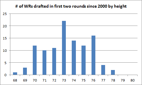
Now, let’s turn to players drafted since 2000. This next graph shows how many wide receivers were selected in the first two rounds of drafts from ’00 to ’13, based on height:

As you can see, the draft is skewing towards taller wide receivers in recent years. Part of that is because nearly all positions are getting bigger and taller (and faster), but the real question concerns whether this trend is overvaluing tall wide receivers.

It’s too early to grade receivers from the 2012 or 2013 classes, so let’s look at all receivers drafted in the first round between 2000 and 2011. There were 21 receivers drafted who were 6’3 or taller, compared to just 14 receivers drafted who stood six feet tall or shorter. On average, these taller receivers were drafted with the 13th pick in the draft, while the set of short receivers were selected, on average, with the 21st pick.

So we would expect the taller receivers to be better players, since they were drafted eight spots higher. But that wasn’t really the case. Both sets of players produced nearly identical receiving yards averages:

Taller wide receivers have fared ever so slightly better than shorter receivers. But once you factor in draft position, that edge disappears. If you look at the ten highest drafted “short” receivers, they still were drafted later (on average, 17th overall) than the average “tall” receiver. But their three-year receiving yards line is better, reading 563-694-790. In other words, I don’t see evidence to indicate that shorter receivers, once taking draft position into account, are worse than taller receivers. If anything, the evidence points the other way, suggesting that talent evaluators are more comfortable “reaching” for a taller player who isn’t quite as good. Players like Santana Moss, Lee Evans, Percy Harvin, and Jeremy Maclin were very productive shorter picks; for some reason, it’s easy for some folks to forget the success of those shorter receivers, and also forget the failures of taller players like Charles Rogers, Mike Williams, Jonathan Baldwin, Sylvester Morris, David Terrell, Michael Jenkins, Reggie Williams, and Matt Jones.

But that’s just one way of answering the question. What I did next was run a regression using draft value using the values from my Draft Value Chart and height to predict success. If the draft was truly efficient — i.e., if height was properly being incorporated into a player’s draft position–then adding height to the regression would be useless. But if height was being improperly valued by NFL decision makers, the regression would tell us that, too.

To measure success, I used True Receiving Yards by players in their first five seasons. I jointly developed True Receiving Yards with Neil Paine (now of 538 fame), and you can read the background about it here and here.

The basic explanation is that TRY adjusts receiver numbers for era and combines receptions, receiving yards, and receiving touchdowns into one number, and adjusts for the volume of each team’s passing attack. The end result is one number that looks like receiving yards: Antonio Brown, AJ Green, Josh Gordon, Calvin Johnson, Anquan Boldin, and Demaryius Thomas all had between 1100 and 1200 TRY last year.

First, I had to isolate a sample of receivers to analyze. I decided to take 20 years of NFL drafts, looking at all players drafted between 1990 and 2009 who played in an NFL game, and their number of TRYs in their first five seasons. (Note: As will become clear at the end of this post, I have little reason to think this is an issue. But technically, I should note that I am only looking at drafted wide receivers who actually played in an NFL game. So if, for example, height is disproportionately linked to players who are drafted but fail to make it to an NFL game, that would be important to know but would be ignored in this analysis.)

To give you a sense of what type of players TRY likes, here are the top 10 leaders (in order) in True Receiving Yards accumulated during their first five seasons among players drafted between 1990 and 2009:

Randy Moss
Torry Holt
Marvin Harrison
Larry Fitzgerald
Chad Johnson
Calvin Johnson
Keyshawn Johnson
Anquan Boldin
Herman Moore
Andre Johnson

First, I ran a regression using Draft Pick Value as my sole input and True Receiving Yards as my output. The best-fit formula was:

TRY through five years = 348 + 131.3 * Draft Pick Value

That doesn’t mean much in the abstract, so let’s use an example. Keyshawn Johnson was the first pick in the draft, which gives him a draft value of 34.6. This formula projected Johnson to have 4,890 TRY through five years. In reality, he had 4,838. The R^2 in the regression was 0.60, which is pretty strong: It means draft pick is pretty strongly tied to wide receiver production, a sign that the market is pretty efficient.

Then I re-ran the formula using draft pick value *and* height as my inputs. As it turns out, the height variable was completely meaningless. The R^2 remained at 0.60, and the coefficient on the height variable was not close to significant (p=0.53) despite a large sample of 543 players.

In other words, NFL GMs were properly valuing height in the draft during this period.

In case you’re curious, the 15 biggest “overachievers” as far as TRY relative to draft position were, in order: Marques Colston, Santana Moss, Brandon Marshall, Darrell Jackson, Terrell Owens, Anquan Boldin, Antonio Freeman, Chad Johnson, Coles, Mike Wallace, Greg Jennings, Chris Chambers, Marvin Harrison, Hines Ward, and Steve Johnson.

In this sample, about 50% of the players were taller than 6-0, and only about 30% of the receivers were 5-11 or shorter. We shouldn’t necessarily expect to see a bunch of short overachievers, but I’m convinced that height was properly valued by NFL teams in the draft at least over this 20-year period. There may be fewer star receivers who are short, but that’s only because there are fewer star receiver prospects who are short. Once an NFL team puts a high grade on a short prospect, that’s pretty much all we need to know.

Of the 33 players drafted in the top 15, just one-third of them were six feet or shorter. As a group, there were a couple of big overachievers (Torry Holt, Lee Evans), some other players who did very well (Joey Galloway, Terry Glenn, and Donte Stallworth), and a few big busts (Desmond Howard, Ted Ginn, Troy Edwards, and Peter Warrick). Ike Hilliard and Mike Pritchard round out the group. But I see nothing to indicate that short receivers who are highly drafted do any worse than tall receivers who are highly drafted. It’s just that usually, the taller receiver is drafted earlier.

Waldman: Why the Exceptional is Valuable

Chase’s analysis echoes what I have heard from those with NFL analytics backgrounds: There are too many variables to consider with raw stats to indicate that big receivers are inherently better than small receivers and there are viable archetypes of the effective small receiver.

What concerns me about the attempts to pigeonhole player evaluation into narrower physical parameters is that if taken too far one might as well replace the word “talent” in the phrase “talent evaluation” and use “athletic” or “physical” in its place. I may be wrong, but I get the sense that some of these Stats Ministers–intentionally or otherwise–dislike the exceptional when it comes to human nature. They’re seeking a way to make scouting a plain of square holes where the square pegs fit neatly into each place.

The problem with this philosophy is that once a concept, strategy, or view becomes the “right way” it evolves into the standard convention. Once it becomes conventional, it’s considered “safe.” However this is not true in the arena of competition. If you’re seeking the conventional, you’ve limited the possibilities of finding and creating environments for the exceptional to grow.

Many players who didn’t match the ideal size for their positions and had success were difference makers on winning teams–often Super Bowl Champions. I’d argue that exceptions to the rule that succeed are often drivers of excellence:

• Russell Wilson didn’t meet the faulty “data backed” physical prototypes for quarterback and picking this exception to the rule in the third round earned them exceptional savings to acquire or keep other players for a Super Bowl run.
• Rod Smith was too short, too slow, a rookie at 25, and not even drafted. But like a lot of his peers I mentioned above, his production was a huge factor for his team becoming a contender. The fact he was the exception to the rule freed Denver to acquire other pieces to the puzzle.
• Joe Montana was too small, threw a wobbly ball, and was a third-round pick who was more of a point guard than full-fledged pocket passer, but he was just the type of player Bill Walsh was seeking in an offense that changed the entire course of the game. But at the time, the west coast offense was the exception to the rule that turned the league upside down.
• Buddy Ryan and the Bears drafted a bunch of defenders that didn’t meet physical prototypes for traditional roles in a 4-3, but the 46 defense took Chicago to Super Bowl dominance.
• Drew Brees, Darren Sproles, and Marques Colston were exceptions to the rule. The Saints offense has been the driver for this team’s playoff and Super Bowl appearances.

I could name more, but the point isn’t to list every player. Why should I? Players who become top starters in the NFL are by very definition the exception to the rule. The only thing height gives a wide receiver is potential position on a target due to wing span, but it doesn’t help hand-eye coordination, body position, route running, comfort with physical contact, and understanding of a defense.

There are also smaller players with good arm length, leaping ability, quickness, and strength to earn similar, if not better position on a target. Even when the smaller receivers lack the same caliber of physical measurements as the bigger players, if they possess all of the other traits of a good receiver that these big athletes lack then size doesn’t matter.

There are legitimate archetypes for smaller, quick receivers with change of direction. However, there are social biases with these correlations that filter out players from the earliest stages of the game. These biases include the idea that the vast majority of these types of players are in the highest levels of football so anything different should be discouraged at the high school and college level–think white wide receivers, running backs, and cornerbacks as examples.

Players who succeed in defying these social biases and also possess the skill and persistence to overcome them. I’ve shown this video before, but physicist Neil deGrasse Tyson makes a strong point against “data backed” arguments of this nature when he answered a question posed about the small number of female and black scientists in the world. Harvard President Lawrence Summers hazarded a guess that it was genetics. Tyson’s answer is a great example why correlation isn’t causation.

The greatest irony about this specific crowd of data zealots is that they are often the first to complain about coaching tendencies that have same biases.

Maybe rookie receivers with the dimensions of Paul Richardson – or for that matter Jeremy Gallon or Odell Beckham – don’t become productive fantasy options or football players as often as bigger players based on correlating data. However, pointing to past history and scoffing at the wisdom of making an investment is like stating that it was a fact in the 15th century that dragons lie at the edge of the flat world we live in.

If you’re going to avoid investing in a player–or encourage others to do so–use good reasoning. Looking at the data is helpful, but the NFL isn’t a perfect data set. There are some data analysts writing about football that derive ideas reliant on a lot of highly fit equations that don’t work in a real world situation. However, they expect perfection and it’s not going to happen. They also behave as if data only tells the truth–and when that data lacks a fit, context, or proper application, it’s a little scary.

I want to see analytics succeed in the NFL, but like film study it’s not the answer. These two areas–when executed well–can contribute to the answer. However, the NFL–beyond some individual cases–hasn’t made significant advances in either area.

I suppose when you have a monopoly in the marketplace combined with a socialistic system for spreading the wealth owners don’t have significant motivation to become innovative with player evaluation. If they did, they’d be spending more money on making these processes rather than cycling through coaches and GMs every 3-5 years.

The Super Bowl is a football competition decided by a series of single-elimination playoff games played after 32 teams attempt to qualify from eight groups of four teams each. That’s the World Cup, too!

And just like the NFL, there are some not-so-good AFC South-ish groups and some very good NFC West-like groups. So let’s assign each World Cup group its doppelganger of an NFL division, and then every team to one of the NFL teams in that division.

That gives us our NFL World Cup Bracket. The AFC South is Group E, which contains no great team and at least one candidate to be the Jacksonville Jaguars of the World Cup. The NFC West is Group B, which has three legitimate contenders to win the whole thing, one of which will not even make it out of the group.

Each team is listed in its predicted order of finish within the group according to my highly scientific NFL-based World Cup prediction machine. Teams with a * are predicted to advance out of the group.

[continue reading…]

Yesterday, I explained the methodology behind the formula involved in ranking every quarterback season since 1960. Today, I’m going to present the career results. Converting season value to career value isn’t as simple as it might seem. Generally, we don’t want a player who was very good for 12 years to rank ahead of a quarterback who was elite for ten. Additionally, we don’t want to give significant penalties to players who struggled as rookies or hung around too long; we’re mostly concerned with the peak value of the player.

What I’ve historically done — and done here — is to give each quarterback 100% of his value or score from his best season, 95% of his score in his second best season, 90% of his score in his third best season, and so on. This rewards quarterbacks who played really well for a long time and doesn’t kill players with really poor rookie years or seasons late in their career. It also helps to prevent the quarterbacks who were compilers from dominating the top of the list. For visibility reasons, the table below displays only the top 25 quarterbacks initially, but you can change that number in the filter or click on the right arrow to see the remaining quarterbacks. ^[1]Note that while yesterday’s list was just from 1960 to 2013, the career list reflects every season in history, using the same methodology as used in GQBOAT IV.

Here’s how to read the table. Manning’s first year was in 1998, and his last in 2013. He’s had 8,740 “dropbacks” in his career, which include pass attempts, sacks, and rushing touchdowns. His career value — using the 100/95/90 formula ^[2]And including negative seasons. is 12,769, putting him at number one. His strength of schedule has been perfectly average over his career; as a reminder, the SOS column is shown just for reference, as SOS is already incorporated into these numbers (so while Tom Brady has had a schedule that’s 0.25 ANY/A tougher than average, that’s already incorporated into his 10,063 grade). Manning is not yet eligible for the Hall of Fame, of course, but I’ve listed the HOF status of each quarterback in the table. Note that I only have quarterback records going back to 1960; therefore, for quarterbacks who played before and during (or after) 1960, only their post-1960 record is displayed. In addition, SOS adjustments are only for the years beginning in 1960. [continue reading…]

In 2006, I took a stab at ranking every quarterback in NFL history. Two years later, I acquired more data and made enough improvements to merit publishing an updated and more accurate list of the best quarterbacks the league has ever seen. In 2009, I tweaked the formula again, and published a set of career rankings, along with a set of strength of schedule, era and weather adjustments, and finally career rankings which include those adjustments and playoff performances.  And two years ago, I revised the formula and produced a new set of career rankings.

This time around, I’m not going to tweak the formula much (that’s for GQBOAT VI), but I do have one big change that I suspect will be well-received.  Let’s review the methodology.

Methodology

We start with plain old yards per attempt. I then incorporate sack data by removing sack yards from the numerator and adding sacks to the denominator. ^[1]I have individual game sack data for every quarterback back to 2008. For seasons between 1969 and 2007, I have season sack data and team game sack data, so I was able to derive best-fit estimates for … Continue reading To include touchdowns and interceptions, I gave a quarterback 20 yards for each passing touchdown and subtracted 45 yards for each interception. This calculation — (Pass Yards + 20 * PTD – 45 * INT – Sack Yards Lost) / (Sacks + Pass Attempts) forms the basis for Adjusted Net Yards per Attempt, one of the key metrics I use to evaluate quarterbacks. For purposes of this study, I did some further tweaking. I’m including rushing touchdowns, because our goal is to measure quarterbacks as players. There’s no reason to separate rushing and passing touchdowns from a value standpoint, so all passing and rushing touchdowns are worth 20 yards and are calculated in the numerator of Adjusted Net Yards per Attempt. To be consistent, I also include rushing touchdowns in the denominator of the equation. This won’t change anything for most quarterbacks, but feels right to me. A touchdown is a touchdown.

Now, here comes the twist.  In past year, I’ve compared each quarterback’s “ANY/A” — I put that term in quotes because what we’re really using is ANY/A with a rushing touchdowns modifier — and then calculated a value over average statistic after comparing that rate to the league average. For example, if a QB has an “ANY/A” of 7.0 and the NFL average “ANY/A” is 5.0, and the quarterback has 500 “dropbacks” — i.e., pass attempts plus sacks plus rushing touchdowns — then the quarterback gets credit for 1,000 yards above average. [continue reading…]

Colin Kaepernick won’t be hurting for weapons this year, which may be why San Francisco decided to give him a massive contract extension prior to the season. So will this be a career year for the young quarterback? Even if he plays well, he may not throw for 4,000 yards due to game script; after all, the 49ers held an average lead 5.9 points last year, and as a result, the team ranked 31st in pass attempts. San Francisco figures to be excellent again, but Kaepernick should produce very strong efficiency numbers in 2014. Assuming they all stay healthy and make the roster, check out the quintet of weapons Kaepernick will have at his disposal:

• Anquan Boldin was dominant for San Francisco last year, and 2013 marked the sixth time in his career he’s topped the 1,000-yard mark. He maxed out with a 1,402-yard season with Arizona in 2005.
• Michael Crabtree was limited to just five games after recoving from a torn Achilles, but he recorded 1,105 yards on a run-heavy 49ers team in 2012.
• Steve Johnson had 1,000-yard seasons in 2010, 2011, and 2012 (with a high of 1,073 in ’10) with the Bills, but will be a 49er in 2014.
• Tight end Vernon Davis has actually never had a 1,000-yard year, but he did gain 965 yards and score 13 touchdowns in 2009.
• Brandon Lloyd may not even make the roster, but the man drafted by San Francisco 11 years ago has seen some success in between his stops with the 49ers.  Two years ago, he gained 911 yards for the Patriots, and in 2010, he led the league with 1,448 receiving yards while playing in Denver.

As of a year ago, only eight teams in NFL history had ever fielded a roster with five players who gained 1,000 receiving yards in a season at some point in their careers. But none of those teams entered a season with five former 1,000-yard receivers: for each of those teams, at least one of the five players had a 1,000-yard season at some point in the future.

But the 2014 49ers would only become the second team to enter a season with five players who had previously gained at least 965 receiving yards in a season. Can you guess the first? [continue reading…]

Every year, I adjust quarterback statistics — both fantasy and traditional — for strength of schedule. Today, a look at my article at Footballguys.com where I adjust the 2013 numbers for each quarterback for the quality of the opposing defenses. On Monday, I’ll be doing the same for quarterbacks using Adjusted Net Yards per Attempt.

For the ninth straight season, I’m advising fantasy football owners about a good starting point for their quarterback projections/rankings. My Rearview QB article analyzes the production of every quarterback from the prior season after adjusting his performance for partial games played and strength of schedule. If you’re a first time reader, here’s my argument in a nutshell: using last year’s regular end-of-year data is the lazy man’s method. When analyzing a quarterback, many look at a passer’s total fantasy points or fantasy points per game average from the prior season and then tweak the numbers based on off-season changes and personal preferences. But a more accurate starting point for your projections is a normalized version of last year’s stats.

The first adjustment is to use adjusted games (and not total games), which provide a more precise picture of how often the quarterback played. Second, you should adjust for strength of schedule, because a quarterback who faced a really hard schedule should get a boost relative to those who played easy opponents most weeks.

To be clear, this should be merely the starting point for your quarterback projections. If you think a particular quarterback carries significant injury risk, or is going to face a hard schedule again, feel free to downgrade him after making these adjustments. (And it should go without saying that if you think a quarterback will improve or decline – or, in the case of Colin Kaepernick or Cam Newton his supporting case will improve or decline – you must factor that in as well.) But those are all subjective questions that everyone answers differently; this analysis is meant to be objective. The point isn’t to ignore whether a quarterback is injury prone or projects to have a really hard or easy schedule in 2014; the point is to delay that analysis.

First we see how the player performed on the field last year, controlling for strength of schedule and missed time; then you factor in whatever variables you like when projecting the 2014 season. The important thing to consider is that ignoring partial games and strength of schedule is a surefire way to misjudge a player’s actual ability level. There’s a big difference between a quarterback who produced 300 fantasy points against an easy schedule while playing every game than a quarterback with 300 FPs against the league’s toughest schedule while missing 3.6 games. Here’s another way to consider the same idea: Jay Cutler ranked 25th in fantasy points in 2013, but the quarterback position for the Bears (i.e., Cutler and Josh McCown) ranked as the 4th highest team QB last year.

You can read the full article here.

It’s no secret that Andrew Luck’s efficiency numbers aren’t quite up to par with his reputation. Over the past two seasons, Luck ranks just 18th in ANY/A, far behind some of the other young quarterbacks in the NFL. Nick Foles, Russell Wilson, and Colin Kaepernick rank in the top 6th in that metric, Robert Griffin is 11th, Cam Newton is 14th, and even Andy Dalton is 16th. Luck tends to fare much better in ESPN’s QBR than in ANY/A (and Andy Benoit wrote an interesting pro-Luck piece yesterday), but today I wanted to try to quantify another issue: quarterback help.

A quick disclaimer: there are probably a zillion different ways to quantify quarterback help. This is certainly not not not the best way, but it’s the way that was easiest and most intuitive to me. On the scale of “this feels right” to “rigorous quantitative analysis” this certainly falls closer to the former end of the scale. But it’s Friday and we’re having fun, so here’s what I did.

1) Calculate how many standard deviations from average each team was in Points Allowed (negative means fewer points allowed).

2) Calculate how many standard deviations from average each team was in Pass Ratio (negative means more run-heavy).

3) Add the two standard deviations to see how much each team relied on each quarterback’s arm.

Here were the 2013 results. According to this, no quarterback was asked to do more than Matt Ryan. Here’s how to read the table below: The Falcons allowed 443 points last year, which was 1.05 standard deviations more than the average team. Atlanta also passed on 68.7% of all plays, which was 1.99 standard deviations above average. Add those together, and the Falcons get a grade of +3.04, the most in the NFL in 2013. [continue reading…]

It’s fun to play with weighted averages to see how the NFL has (or hasn’t) evolved. For example, the Giants led the league with interceptions: as a result, 5.8% of all interceptions thrown in the NFL last year were by Eli Manning or Curtis Painter. Since the Giants went 7-9 in 2013, that means 5.8% of all interceptions were thrown by a team that had a 0.438 winning percentage. Meanwhile, Kansas City and San Francisco each threw just 8 interceptions, or 1.6% of all NFL interceptions, and the Chiefs and 49ers had an average winning percentage of 0.719.

So while the average winning percentage of all NFL teams is of course 0.500, the average weighted (by interceptions) winning percentage of all NFL teams will be below .500 because bad teams tend to throw more interceptions than good teams. Last year, the averaged weighted winning percentage was 0.464 for all NFL teams.

What’s interesting is how little variation there has been over the years in weighted winning percentage. In fact, it’s been between 45% and 50% in just about every year since 1950: [continue reading…]

Josh Gordon led the league with 1,646 receiving yards last year. That’s impressive: perhaps even more impressive is that he did it on “only” 159 targets, meaning he averaged 10.35 yards per target. ^[1]That’s the most of any receiver with over 130 targets. It’s the second most among players with 100 targets, behind DeSean Jackson‘s 10.6 average on 126 targets. It’s the … Continue reading But the most impressive part, of course, was that he did it for the Browns. You know, the Browns, quarterbacked by a three-headed monster of Jason Campbell, Brandon Weeden, and Brian Hoyer, each of whom managed to average a around the same mediocre 6.4 yards per attempt.

Here’s another way to think of it. While Jordan Cameron was somewhat efficient (7.7 yards per target), the other three Browns to finish in the top five in Cleveland targets were Greg Little (4.7 yards per target), Chris Ogbonnaya (4.6), and Davone Bess (4.2!). And here’s yet another way to think of it: the Browns threw 681 passes last year and gained 4,372 passing yards. But 1,646 of those yards came on the 159 passes intended for Gordon. Remove those plays, and Cleveland averaged just 5.22 yards per pass attempt on passes to all other Browns last year.

That means Cleveland averaged 5.13 more yards per target on passes to Gordon in 2013 than on passes to everyone else. That’s insane, particularly over 159 targets. How insane? If we multiply those two numbers, we get a “value relative to teammates” metric: Gordon gained 816 more yards on his targets than the other Browns averaged per target. Now, in the abstract, maybe 816 doesn’t mean much to you. But it’s the most of any player since at least 1999. The table below shows the top 75 wide receivers in value relative to teammates: the columns should be self-explanatory, and the “ROT Y/A” shows the yards per attempt on passes to the rest of the team. As always, it’s fully sortable and searchable; by default, it displays only the top 25 receivers, but you can switch that by clicking on the dropdown box to the left. [continue reading…]

Last week, I wrote about whether having great college teammates might cause quarterbacks and wide receivers to be overvalued in the NFL draft. The results were inconclusive on the impact of teammates on quarterbacks, but they indicated that wide receivers who played with first-round QBs in college tended to underperform in the NFL relative to their draft position. Receivers such as Mike Williams of USC (#10 in 2005) and Marcus Nash of Tennessee (#30 in 1998) may have gone too high in the draft in part because they played with great college QBs who made them look good.

Today, I look at running backs drafted since 1984. I use a slightly different way of looking at the data that I think is a little better. I also revisit the QBs and WR/TEs with that method. Instead of considering the number of first-round college teammates that a player has, I consider the total draft value of college teammates at different positions, as determined by Chase’s chart. ^[1]I thank commenter Stuart for suggesting this approach in the comments to last week’s post. Going this way makes it possible to look at the entire offensive line’s value, for example, rather than just the number of players who were high picks.

For example, according to PFR’s Approximate Value (AV), Ki-Jana Carter is the biggest underachiever at RB relative to his draft position (since 1984). After being drafted #1 in 1995, he generated just nine points of AV in his first five years. ^[2]Carter averaged 3.3 yards on 227 carries over his first five injury-plagued seasons. Carter also had a lot of help from his friends in college. He ranks 10th out of 104 RBs picked in the top 32 in terms of the total value of his college offensive linemen according to my measure. His tight end also went in the top ten in 2005; Carter would be 2nd in total line value if we included TEs. Two of his offensive lineman went in the first round in the following year. Two Penn State fullbacks were drafted that year, too. ^[3]Two Penn State halfbacks were drafted in 1996, as well. One of them was Stephen Michael Pitts, who went to Middletown High School South (NJ), a school that also graduated Knowshon Moreno and, only … Continue reading Could Carter have looked better than he was because he ran behind those great college blockers? Or is the NFL success of the running back who ranks fourth in terms of offensive line help (Warrick Dunn) more representative of RBs, in general?

In addition to looking at the offensive line, I’ll consider whether the total value of college teammates at other offensive positions predicts that running backs become overvalued in the draft. While we might think that RBs are particularly dependent on line help, it actually appears that having a great QB is again the one clear predictor for players being overvalued. [continue reading…]

Comparing wide receivers across teams is tricky. Pierre Garcon led the NFL in targets, ^[1]All target data comes courtesy of Footballguys.com. but that’s partially because Washington didn’t have much help at wide receiver. ^[2]And in the offseason, Washington signed DeSean Jackson and Andre Roberts Vincent Jackson was 2nd in percentage of team targets (we’ll get to who was first in a few minutes) for a similar reason: Jackson is a very good receiver, but Tampa Bay had limited weapons in 2014. ^[3]And in the 2014 NFL Draft, the Bucs added Texas A&M wide receiver Mike Evans and Washington tight end Austin Seferian-Jenkins. At least in theory, the high target numbers for Garcon and Jackson should be considered in light of the fact that both teams had below-average passing offenses.

The flip side of that coin is a player like Demaryius Thomas. In 2012, while “competing” with another very good receiver in Eric Decker, Thomas saw 24.2% of Denver targets.  Last year, with the addition of Wes Welker and a breakout season from Julius Thomas, Thomas saw just 21.2% of Broncos targets. But the team’s passing game was better, so arguably Thomas should receive a “bump” in his target percentage because he played for a great offense.

That’s just in theory. The unspoken elephant in the analysis is the quarterback. It’s not just a player’s supporting cast of weapons that determines whether his team has a good or bad passing attack: Thomas obviously benefited greatly from playing with Peyton Manning, too. Regular readers may recall that last year, for each team’s leader in targets, I compared their target percentage (defined as targets divided by all team targets) to their team’s passing efficiency (defined by Adjusted Net Yards per Attempt). I thought it would be fun to perform the analysis again, even if it may make more sense in theory than in practice. Take a look: the Y-axis shows percentage of team targets, and the X-axis respects Team ANY/A. In theory, the best WR1s should be up and to the right, with the worst WR1s (or tight ends masquerading as WR1s) in the bottom left corner of the chart.

[continue reading…]

Over the last three years, Calvin Johnson has 5,137 receiving yards in 46 games.  That’s an average of 111.7 receiving yards per game, the most by any player over a three-year stretch in NFL history.  That mark comes with a bit of an asterisk, of course, as the Lions have attempted 2,040 passes since the start of the 2011 season, also an NFL record; that’s why I like using True Receiving Yards and various other WR Ranking Systems rather than just raw receiving yards.

But hey, trivia is trivia, and Johnson is the current record holder.  But prior to 2013, do you know who held the record for receiving yards per game over a three-year stretch? The answer is not Jerry Rice, or else this would be a really lame trivia question.  Rice averaged 101.0 receiving yards per game from 1993 to 1995, and is one of just three players to average over 100 receiving yards per game for a three-year stretch.  Megatron also averaged 101.4 receiving yards per game from 2010 to 2012, but he only became the 3-year king after the conclusion of the 2013 season.

I suspect you’ll also be surprised to see who would is number 4 on the list of most receiving yards per game over a three-year span (counting each player only once, of course).

[continue reading…]

References

1 These perverse incentives have been going on a long time, too. Check out Michael Lewis’s Liar’s Poker for fascinating stories of investment bankers pushing junk on their clients.
{ 18 comments }
The top passing game of 2013
The top passing game of 2013.